Deep Learning-4-3 Generative Models

Learning Objectives

• PixelRNN & PixelCNN
• GANs: Generative Adversarial Networks
• VAEs: Variational Autoencoders

---

In this lesson, we’ll talk about a different class of unsupervised learning methods called generative modeling. Here we take a probabilistic view of unsupervised learning and try to estimate the probability distribution over the input space.

In unsupervised learning, there’s a whole host of different tasks we may want to do. In this lesson, we’ll focus on Density Estimation, that is producing a model of the probability distribution over the input space. In some cases, we may want to just have the ability to generate samples from this distribution, that is actually generate artificial examples that come from this distribution.

Recall the distinction between Discriminative and Generative models:

• Discriminative models, model the conditional distribution probability of the label given the input. Examples of this include neural networks, support vector machines, random forests and so on. You may not have known that this is actually what we’re doing, because really we just approximate this probability distribution using a blackbox neural network. We haven’t done any additional probabilistic reasoning. However, if you’ve taken a machine learning course, you may have learned that there’s an entire probabilistic and statistical view of machine learning. Where we can actually write out these probability distributions and reason about them. For example, to derive what loss functions we may want to use.

• Generative models, on the other hand, models the distribution over the input space. Now, this is a very complex distribution, and so there’s a question of how we can actually model it. Just, like discriminative models we can have a parametric approximation of this distribution. That is we can have a set of parameterized models $p(x,\theta)$. And use the principle of maximum likelihood to optimize the parameters given the unlabeled data set. Here $p(x,\theta)$ is our likelihood and we wanna maximize it or are real theta, that is we want our model to output high probabilities for the real deta. We can use this as the optimal set of parameters, data star, being the argmax data of the product of the likelihood of each example. This is because the examples are drawn independently and identically, that is we’re just sampling independently from this distribution. And so the likelihoods of all of the data can be decomposed as the product of the likelihood of each piece of data. We can then take the log of this because we’re maximizing it, and this turns out into a sum of log likelihoods.

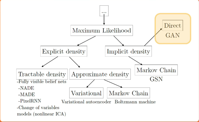
These are called generative models because they can often generate samples. Once, we have some parameters data, we can also generate examples from this distribution that we’re approximating. Some examples include multi-variate Gaussian model, where we have mu and sigma, that is the mean and co-variants. And what we wanna do is estimate these values from the data, and then given these estimates, we can just sample from the multi-variate Gaussian to actually produce example. Now, of course, this is very difficult, especially for high dimensional data. Because generative modeling is so difficult, there’s been a whole host of different methods that have been developed. These can be categorized in various ways, for example, whether they use the maximum likelihood principle in order to optimize their parameters. There are methods that perform explicit tractable density estimation. That is, they simplify the joint distribution into some factorized model consisting of simpler components and then learn parameters for those. There are methods that perform approximations of various kinds, that is, they learn distributions that approximate the true joint distribution. And then there are implicit density models, where we don’t actually model the density itself. Rather, we’re just able to perform tasks such as sampling from the density. That is we can generate samples from the probability distribution, but we can’t really have an explicit model for it that we learned. We’ll cover the three most popular methods across the spectrum, in order to give you a flavor of all the different methods that exist.

PixelRNN & PixelCNN

In this lesson, we’ll talk about generative models that perform explicit tractable density estimation, that is still reduce or factorize the joint distribution into something that’s much more manageable that we can then approximate or learn using a recurrent neural network or CNN.

The first set of models that we’ll talk about represent the joint distribution as an explicit tractable density. This is going to be similar to methods such as language model, where we model the distribution over sentences as just the product of the likelihoods over the work. We’ll do something similar, for example, for pixels in images. To simplify matters, we can use the chain rule to decompose the joint distribution. ie factorizing the joint distribution into a product of conditional distribution.

Mathematically:
$$
\large p(x) = \prod_{i=1}^{n^2} p(x_i|x_1,\cdots,x_{i-1})
$$

In the context of language modeling, this should be familiar. Rather than modeling the joint distribution over all words in a sentence, we can just factorize it, and here we have a natural sequence or ordering because the words come in a word at a time. And so we can model the probability of the sentence as the product of the conditionals, the probability of the first word, the probability of the second word given the first word and so on. And we can just take the product of these likelihoods in order to model the probability of the sentence.

Mathematically:
$$
\large p(S) = p(w_1) p(w_2|w_1) p(w_n|w_1,\cdots,w_{n-1}) = p(w_1,w_2,\cdots,w_n)
$$
We can do something similar with images, here rather than the basic unit being words, the basic units are pixels. We can factorize the joint distribution as the product of conditionals, where we define some ordering over the pixels. For example, we could start with just the upper left pixel, and have some prior probability distribution over that pixel value. We can then move to the subsequent pixels from left to right and top to bottom, we can then model the probability of x as equal to the probability of x1, the upper left pixel times the probability of x2 given x1 times the probability of x3 given x1 times the rest of the product.

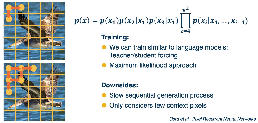
We can also do student forcing, where the model predicts some distribution over the pixel values for this current pixel, and then we use the conditional as that value for the next pixels. Over time, we can then train this across the entire image and we’re updating our model to be better and better at modeling this conditional distribution p(xi) given the prior pixels. Once we have the model trained, we can actually generate new images, just sample from p(x1) that is the prediction of the model for the first pixel and then use that as input to predict the next pixels and sample from that.

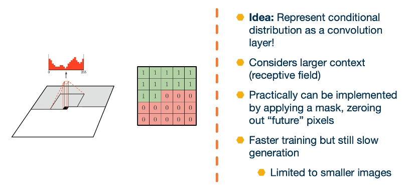
Another idea is to represent the conditional distribution as a convolution, that is rather than conditional on just the adjacent pixels, we have a receptive field or a window and then we have a learnable convolution filter that output this distribution. The downside is that there’s some future pixels that is part of the convolution window that we may not know.

GANs: Generative Adversarial Networks

In this lesson we’ll talk about a different class of generative models called generative adversarial networks. Generative adversarial networks or GANS did not learn an explicit density function p of x, rather they fit under the implicit density category. What that means is rather than learn a parameterised density function We will instead learn a parameterised generation process that can give us samples from the joint distribution.

We won’t have an explicit density though, to perform things like classification or things like that. But we’ll still be able to use the unlabeled data to learn how to generate new samples. That fits that distribution of the unlabeled data, or even learn features that might be good for downstream tasks.

First we have to learn how to sample from a neural network output. It’s not clear how to produce random outputs. Given some fixed input thus far, we’ve only dealt with a particular input and then generate a particular output. We also will use the notion of adversarial training. We’ll use one that works predictions to train another networks, lost function. This is essentially can be seen as a dynamic loss function and you have two neural networks learning at the same time that we will pit against each other.

There’s also lots of tricks to make this more stable. Because you have a game theoretic optimization pitting two neural networks against each other, the complex dynamics of learning will actually turn out to be quite difficult to train. And so there’s a lot of different tricks that researchers have developed in order to make this more stable and effective.

Suppose we would like to sample from a very complex distribution p(x) using a neural network. We’re going to use a simple idea of first sampling from a simple distribution, they a Gaussian, where we know how to generate samples from, and then we’ll actually learn a transformation function that transforms samples from that simple distribution to samples from the complex distribution. Here’s an illustration.

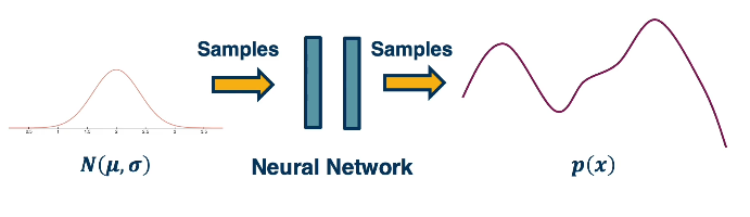
Now this transformation function can be pretty complex, but that’s okay. We have deep learning where we can learn really complex functions as a result.

Here’s a concrete instantiation of this idea:

• Suppose we sample from a Gaussian many different times to generate a vector of independently generated random numbers
• then we take this vector and use a generator that is a network that takes a vector and up samples into an image
• or transforms it into an image through a complex set of convolutions and spooling layers
• then it outputs a complete image.

The key idea of generative adversarial networks is to have another network that distinguishes between real and generated or fake images. And the reason we wanna do this is that how well the discriminator performs, can be used as a signal to determine how well the generator is doing.

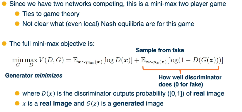
Here, the discriminator is supposed to output a probability of one for the real image and zero for the fake image. And so if d of g of z should be zero, because it’s a fake image, then we want one minus d of g of z. And then we take the log of that. And so this is essentially saying how well does this discriminator going to do? And the generator wants to minimize this because the generator wants to fool the discriminator.

So again, this right side of the objective function is saying how well is the discriminator doing on fake data and generator wants to minimize that because it wants the discriminator to not do well. Note that the objective function for the generator only is affected by the right side. That is the gradients for the first part of the term of the objective function is zero. Because if you notice it only has log of D of x and there’s no term there that depends on G. So no amount of changing G parameters will affect that part of the objective.

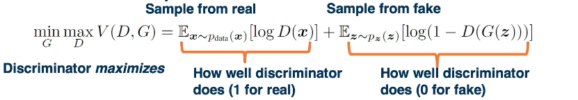
On the other hand, the discriminator is doing the opposite. We can sample from the fake data and the discriminator wants to maximize this, how well the discriminator does, that is, it wants to output zero for the fake data. At the same time we sample a mini-max from the real and again the discriminator is maximizing this Note that for the generator, only one part of this objective function is valid. On the left side of the objective, we just have [log of D(x)]. That is the discriminator output on real data. And nothing we change about the generator’s parameters effects this part of the objective That is a gradient zero.

So really the gradient for the generator only comes from the right side of the term, whereas the gradients for the discriminator comes from both. It wants to both do well on the real as well as on the fake in discriminating them.

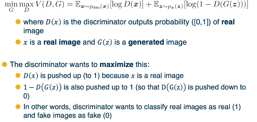
Recall however the generator’s wants to minimize

• 1-D(G(z)) will be pushed down to 0 while D(G(z)) will be lifted to 1
  • this means that it is taking fake data and giving it a probability of being real as 1
• This means that the generator is fooling the discriminator
  • ie succeeding at generating images that the discriminator can’t discriminate from real

So again, we’ll update the generator using the gradients from this objective. So we’re tuning both the generation process and the feature extraction in order to essentially output more and more realistic images. Here is a visual depiction of the same thing.

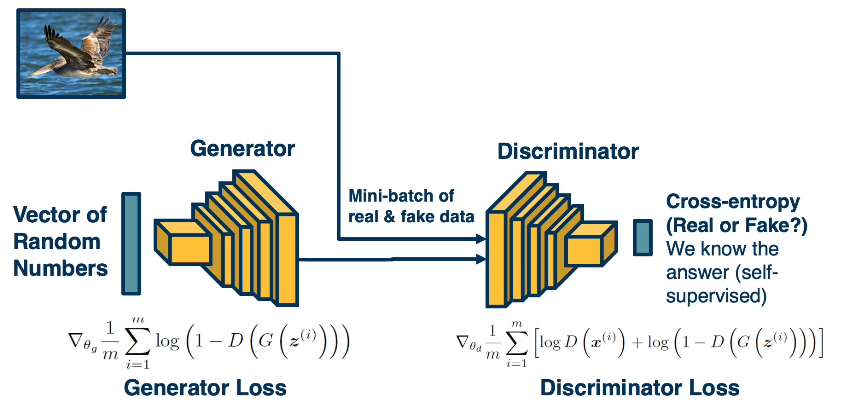
Again, we’ll have a mini batch of real and fake data, we’ll have the generator producing the fake data, where we start from a vector of random numbers, where each random number in the vector is sampled from a normal distribution. And then we’ll also have in the mini batch real images. And we’ll feed those discriminator, and each part will have an objective, the generators objective only touches the 1-D(G(z)), because that’s the only part of the objective that has G in it. And we’re going to average this over the mini batch, that is over the fake data in the mini batch.

The discriminator loss on the other hand, includes both of the terms it wants to both make sure that it outputs a high probability for the real data and a low probability for the fake data. And so we’ll perform backprop and average the gradients over the entire mini batch. And it turns out that the generators part of the objective is actually not very good in terms of its gradient property.

VAEs - Variational Autoencoders

In this lesson we’ll talk about variational autoencoders. Another type of generative model that actually maintain explicit density models, as well as have some approximation that allow us to actually train them in a tractable manner.

These are explicit density models, which have approximate densities. And in this case the optimization itself is approximate.

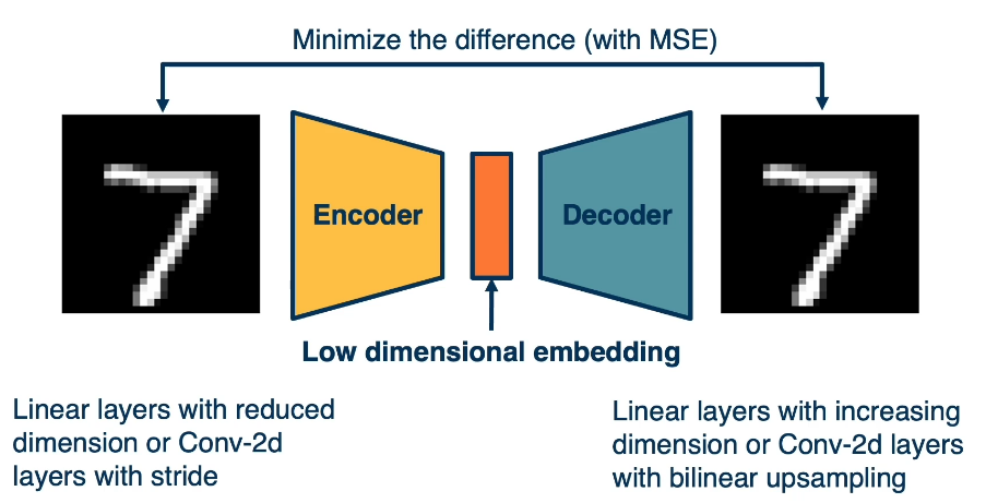
Recall that autoencoders are architectures where the input is fed through an encoder, in order to generate a low-dimensional embedding. And this low dimensional embedding or bottleneck is then used in the decoder in order to reconstruct the image. A loss function (such as mean squared error) can be used in order to minimize the difference between the input and the reconstruction. The actual bottleneck features are hidden or latent variables. What we’d like them to be is disentangled factors of variation that produce an image.

For example, in the case of handwritten digits, it can be what digit it is. The orientation, the scale and so on. Again, the key idea is that there exists some low dimensional set of factors that determine how the image is generated.

We can actually write down an equation for the likelihood that involves these latent variables which we call z(orange middle bar in image), specifically, we can marginalize out the Z.
$$
P(X)=\int P(X|Z;\theta)P(Z)dZ
$$

So P of x can be just the integral of p of x given z here, also including theta, since it’s the parametric model that we’ll use times P(z), that is the prior over z times dz. Now, if we could directly maximize this, then we’re essentially maximizing the likelihood and optimizing the parameters. But we can’t really do this. Instead we maximize a variational lower bound (VLB) that we can compute.

The notion of variational autoencoders combines a set of ideas, including

The notion of variational autoencoders combines a set of ideas, including

• a probabilistic view of generative models
  • where we have P(X), in this case P(X|Z), some latent variables, and we try to use maximum likelihood to optimize the parameters,
• notion of sampling where we’ll actually sample z from a random distribution.
• The notion of auto encoders, rather than having just the decoder,
  • which we’ll have in other models will also have an encoder that actually takes an image and estimate the Z.
• then we’ll also have approximate optimization, which we’ll talk about.

Just as before, we’ll start with a Z vector, where we sample from a random z in this case and then feed it through a decoder. And again this decoder models are P(X|Z) with some parameters.

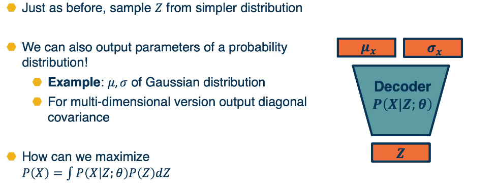
And here the output rather than being just the image for example, it will be a Gaussian distribution parameter. Here specifically, it will be mu and Sigma. That is the mean and covariance matrix of the distribution. We show them as vectors here, but they can just as well be images. And we know that for multi-variate Gaussian outputs, we’re not actually going to output a complex, large covariance matrix. We’re just going to output the diagonal covariance. We’re going to assume that the different dimensions are independent. So, this is essentially nothing but a decoder that rather than outputting deterministic thing, it outputs a set of parameters for a simpler distribution that we know how to sample from, for example, a Gaussian. So given a Z vector, we can feed it through the decoder, it gives us some mu and sigma. And if we actually want to generate samples, we just sample from this Gaussian instead.

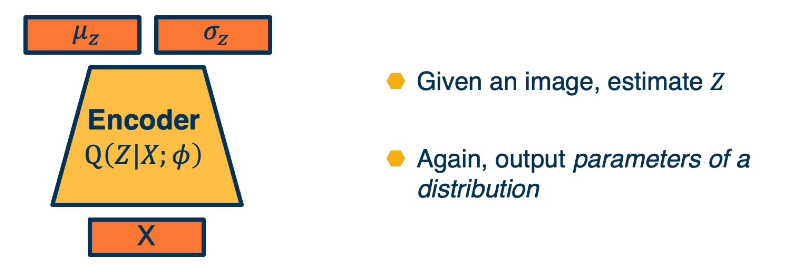
The problem still remains. How can we maximize the likelihood for this model? And it turns out that if we also have an encoder, then actually we’ll be able to derive some gradients that actually do quite well. In this case, we’ll have an encoder, where given an image will have Q of z given x with again, some new parameters ϕ. So this is a different model than the decoder. And again given x, it’ll output not a particular z but it will output the parameters of a Gaussian distribution mu and sigma. And if we wanna generate an actual z, we again just sample from this simpler Gaussian. So now we have both an encoder and a decoder. We can put the encoder and decoder together that is given real data. Again, the whole idea of all of these generative models is that we have samples from the distribution and we want a model P(X).

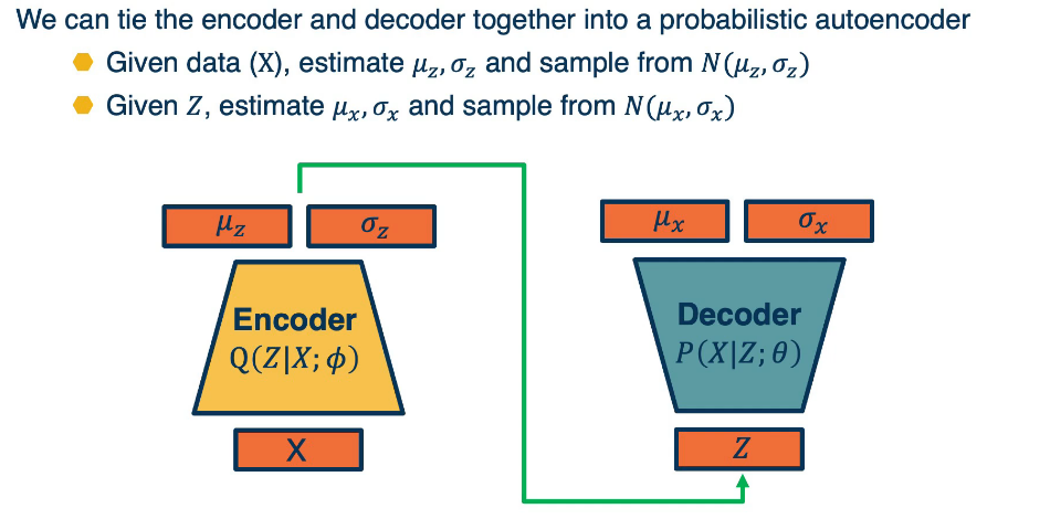
So given a piece of data X or a mini batch of data, we’ll estimate mu and sigma and then sample from that normal distribution to generate Z. Given Z’s, we can then feed it through the decoder. And then we can again estimate mu and sigma for x and then sample from that to generate samples. Again, if we want to use a standard straightforward autoencoder loss, we can just compare the reconstructed x with the original x, but in this case, we’ll have a more sophisticated derivation of a loss function.

And so the question remains, How can we optimize the parameters of the two networks, the encoder and the decoder? Again, we’re going to use the principle of maximum likelihood just write out the term for log of probability of xi where xi is a sample. What’s interesting here is that, since we have an encoder that can take a particular xi produce mu z and sigma z and actually sample from that Gaussian in order to produce z samples. We can actually write this out as an expectation over q of z given x of the log probability of xi. One thing to note here is that the probability of xi doesn’t actually depend on z.

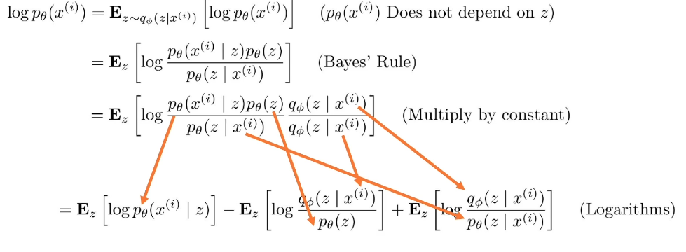
What’s interesting to note is that the expectations that we get on the right side, the two terms on the right are actually equivalent to a similarity measure called KL divergence. As an aside, KL divergence is a distance measure between probability distributions.

And we saw this being used. For example, to derive why we use the cross entropy loss. One thing to note is that it’s always greater or equal to 0. So if two probability distributions are exactly the same, we’ll have a KL divergence of 0, whereas if they’re different than it can be unbounded. The equation is as follows, H denotes the entropy

$$KL(p||q)=H_c(p,q)-H(p)=\sum p(x)log p(x) - \sum p(x) log q(x)$$

Recall that $E[f]=E_{x\sim q}[f(x)]=\sum q(x)f(x)$

So we can rewrite KL as $KL( q(z) || p(z|x) ) = E[log q(z)] - E[log p(z|x)]$

Now let’s use this in our derivation from earlier

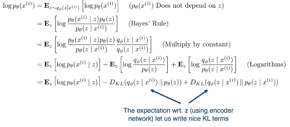
Explanation:

Term 1 :

• Decoder gives us pθ(x|z) so we can compute an estimate of the term through sampling
• and sampling is differentiable through a reparametrization trick
• http://gokererdogan.github.io/2016/07/01/reparameterization-trick/

Term 2 :

• This KL term (between gaussians for encoder and z prior) has nice closed-form solution

Term 3 :

• We cannot compute this as pθ(z|x) is intractable as we saw earlier
• but we do know that the KL must be greater than or equal to 0 so this will suffice

We can’t compute term 3, so what we’re going to do is do basically just ignore it. We know that KL divergence is always greater or equal to zero. And so if we just maximize the first two terms here, we know that we’ll still be making progress.

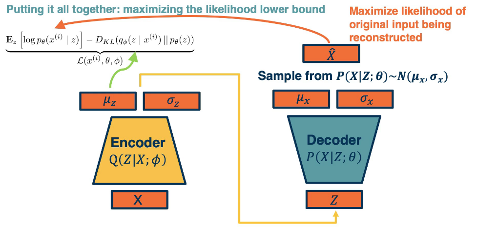
let’s summarize how we can train our variational autoencoder. We’ll have a mini batch of unlabeled data x, and we’ll run it through our encoder. Q(Z|X;ϕ) this will be used to output parameters of a Gaussian distribution. Again, this is an assumption we make mu z and sigma z. And so we’re going to make the approximate Posterior distribution close to the prior. That is we’re going to take the KL divergence between Q of z given x, which is what we’re computing here, and P of z. Again this can be assumed to be a normal distribution, let’s say with a mean of zero and standard deviation of one for example, and this is a KL divergence between two Gaussian distributions which actually can be computed in closed form. We can then sample from this and generate a bunch of Z. And then we feed it through our decoder, which feeds it through P of X given Z with parameters theta and generates mu X and sigma X. And now we can essentially maximize the likelihood of the original data being reconstructed. That is we’re going to maximize the log p of x given z, which is what our decoder is computing here.

Finally we can put it all together in a single picture: