Deep Learning-4-2 Unsupervised and Semi-Supervised Learning

Learning Objectives

• Semi-Supervised Learning
• Few-Shot Learning
• Unsupervised and Self-Supervised Learning

---

In this lesson, we’ll go beyond supervised learning and talk about various other machine learning settings. For example, we’ll look at low labeled machine learning settings where we have only a few labeled examples, possibly with a larger amount of unlabeled example. We’ll also talk about pure unsupervised or self-supervised learning where we’ll try to learn effective feature representations using unlabeled data only.

We will be looking at three main types, but there are many more

• In semi-supervised learning, we have some reasonable amount of labels per category, let’s say ten or more. However, we also have a large set of unlabeled data.
• In few-shot learning, this is taken to extreme. Specifically, we have only 1 to 5 examples per category. In the vanilla setting, we also don’t have any unlabeled data, but it is assumed that we have some larger labelled auxiliary set. What we wanna do is learn models and feature representations that will generalize or transfer to a new set of categories where we only have 1 to 5 examples per category.
• In self-supervised learning, which is a form of unsupervised learning, we assume we have no labels.

Note that in traditional machine learning, and to some degree in deep learning, there’s also purely unsupervised learning where we can perform tasks, such as clustering or density estimation. We’ll talk about the distinction between self-supervised and unsupervised learning later.

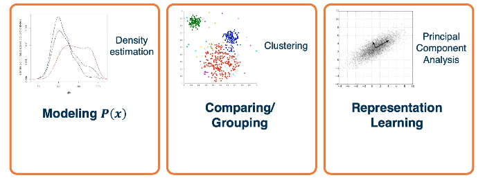
For modeling the P(x), there are deep generative models. For comparing and grouping, there are metric learning, or clustering approaches. And obviously, representation learning is pretty much what deep learning is.

Some Common ideas are shown below.

For modeling the P(x), there are deep generative models. For comparing and grouping, there are metric learning, or clustering approaches. And obviously, representation learning is pretty much what deep learning is.

Semi-Supervised Learning

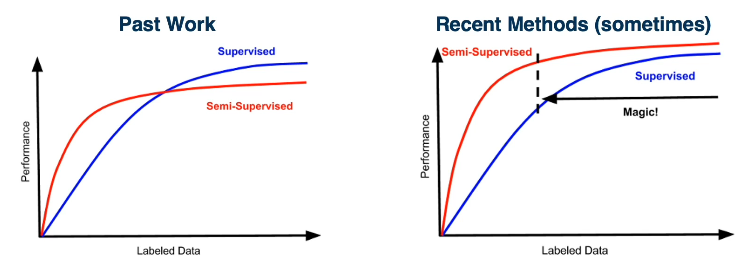
It is often much cheaper (cost/time) to get large-scale unlabeled datasets. This begs the question: Can we overcome a small set of labeled data by using unlabeled data? Which is often much cheaper to get in a large scale (such as the internet). Further, would it improve the performance all the way to a highly labeled scenario?

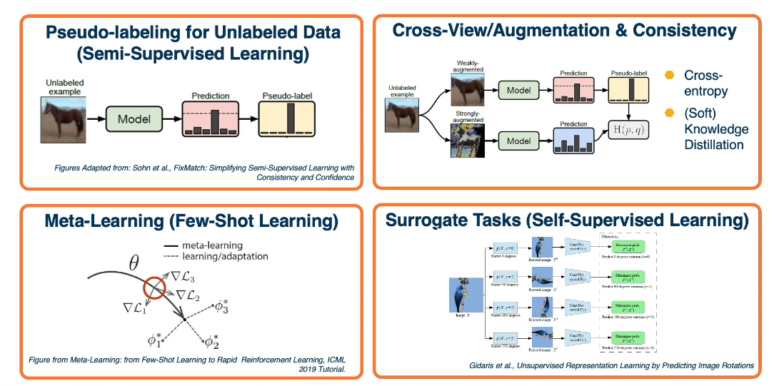
A very simple idea is to learn/train a model on labeled data, make predictions on unlabeled data, then add back into the training data. This can be repeated as often as is necessary. Another approach is to combine unlabeled and labelled data and perform co-training predictions across multiple views. In this method we generally use augmented data techniques.

There is a recent algorithm called FixMatch(https://arxiv.org/abs/2001.07685). Which has proven extremely effective in the Semi-Supervised Learning context. There are several ways to instantiate this idea. There would be two stages where we train the supervised model on the label data. And then we apply that model on unlabeled data. Obtain pseudo-labels for those predictions that are confident, feed those back into the training set. Again, we’ll retrain the supervised model.

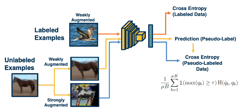
The beauty of deep-learning is that we don’t actually have to do this in multiple stages. We can have this entire pipeline trained in an end to end manner. Specifically, we can have the mini batch consist of both labeled and unlabeled examples. For the labeled part of the mini batch, it goes through the traditional pipeline. We’ll extract features, make predictions and then use cross-entropy loss because we have ground truth labels annotated by humans. For the unlabeled examples, we’ll apply two types of augmentations. Again do feature extraction and prediction. And then use the predictions obtained on the weakly augmented labeled data, not in its own loss functions, but really as ground truth for the loss from the strongly augmented data. At the bottom right we can see what the loss function looks for the unlabeled part. We’ll have a batch size B, for example, 64 examples for the labelled part. And then we’ll have a multiplication factor here, for example 7. So our unlabeled mini batch size will actually be much larger than the labeled part. Finally, we just sum up the loss function and averages. And our specific loss function will include the cross-entropy loss H, between the pseudo-label Q hat B and our predictions from the strongly augmented data QB. And then we’ll also have this indicator function, which looks like a 1, that only applies this to the predictions that have some greater than a threshold prediction.

Some details to keep in mind

• Labelled data batch size of 64, and Unlabeled batch size of 448 is a key factor
• Confidence threshold of 0.95
  • too low and the pseudo labelling will be noisy
  • this causes weight convergence difficulties
• Cosine learning rate schedule
  • $\large \eta cos(\frac{7 \pi k}{16 K})$
• These can differ though for larger data sets
  • batch sizes (1024/5120)
  • Confidence 0.7
  • Inference using the EMA of weights
    • $\theta’t = \alpha \theta’{t-1} + (1-\alpha)\theta_t$

While Fixmatch is the most recent there are other methods

• MaxMatch/ReMixMatch is a more complex variation prior to fixmatch
  • uses temperature scaling and entropy minimazation
  • Multiple augmentations and ensembling to improve pseudo-labels
• Virtual Adversarial Training
  • Augmentation through adversarial examples (via backprop)
• Mean Teacher:
  • Student/teacher distillation consistency method with exponential moving average

Few-Shot Learning

In this lesson we discuss few shot learning where you may only have a few examples per category. Furthermore you may, or should, have a larger model from which you can transfer some learning, but which may have been built for some other purpose. The goal of few-shot learning is to learn a new capability from a very small number of examples.

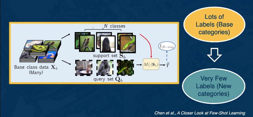
In most literature on few-shot learning the approach is studied in terms of N-Way-K classification. Here the goal is to discriminate between N classes with K examples of each. For ex 10-5 would imply 10 classes with 5 samples a piece.

Some approaches include:

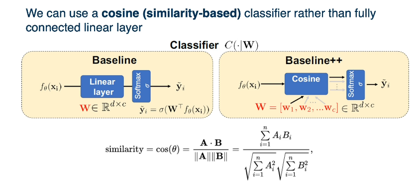
• Fine-Tuning
• Train classifier on base classes
• Optionally freeze the feature extractor
• Learn classifier weights for new classes using a few amounts of labeled data during query time
  • this is surprisingly effective compared to more sophisticated methods

Interestingly a cosine layer (rather than a simple fully connected layer) has been shown to be beneficial in many situations but not all.

There are some drawbacks

• The training we do on the base classes does not factor in the task into account
• No notion that we will be performing a bunch of N-way tests, during inference time

One positive note is that it simulates what is seen during test time. This leads us to the idea of Meta-Learning. In the meta-learning framework, we learn how to learn to classifiy given a set of training tasks and evaluate using a set of test tasks. In other words, we use one set of classification problems to help solve other unrelated sets.

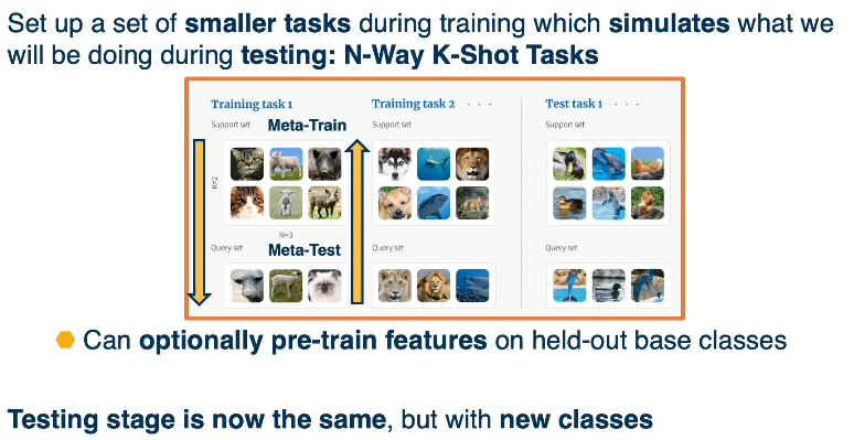
The key factor here is that the classes shown are different than anything seen before.

This begs the question: What can we learn from these meta learning tasks, and what models can be constructed and conditioned on a support set M(⋅|S).

We can think of this as parametrizing a learning algorithm.

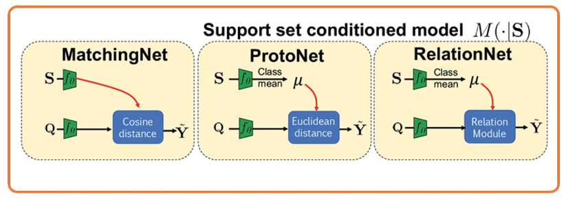
There are Two main aproaches to defining a meta-learner:

• Be inspired from a known algorithm
  • kNN/Kernal machine: Matching Networks
  • Gaussian Classifier: Prototypical Networks
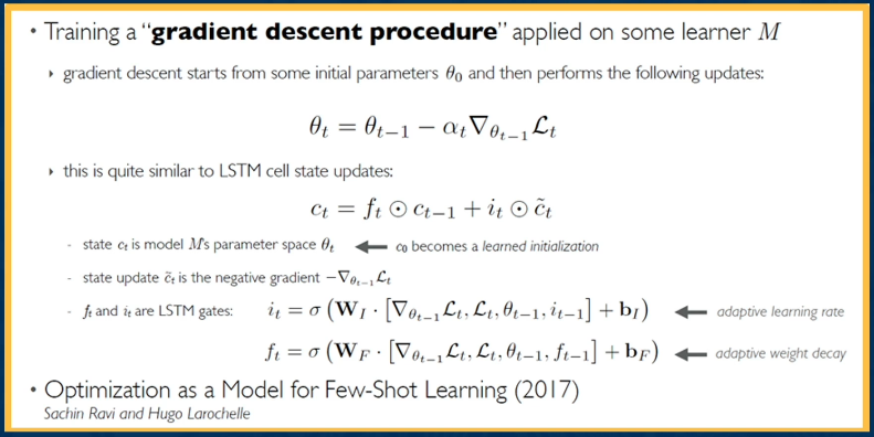
  • Gradient Descent: Meta-Learner LSTM (Model agnostic Meta Learning MAML)
• Derive is from a black box neural Network
  • MANN ( Santoro et al 2016 )
  • SNAIL ( Mishra et al. 2018 )

For example if we wanted a model to learn gradient descent.

• Input: Parameter initialization and update rules
• Output: 1). Parameter initialization 2). Meta-Learner that decides how to update parameters

Meta-Learner LSTM

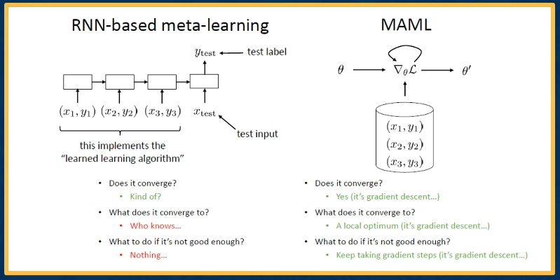
Contrast between MAML and RNN(LSTM) based meta learning methods

Unsupervised and Self-Supervised Learning

In this lesson, we’ll talk about unsupervised and self supervised learning, where we have only unlabeled data, and we’d like to learn effective feature representations, so that we can fine tune them for downstream tasks.

In supervised learning, we have explored a number of architectures and last function in order to optimize this task.

• Classification, we often use fully connected networks at the end, which are then converted to probabilities through softmax, and we use the cross entropy loss.
• Regression tasks, we can use other loss functions, such as mean squared error. The key is that we have labels and these labels allow us to compute these loss functions, and we can use that to back propagate through the network to update the parameters.

In unsupervised learning, there’s a set of traditional tasks that we may want to perform.
For example:

• We may want to perform clustering where the output is a set of clusters or groupings of data, where similar pieces of data are grouped into the same cluster, and this similar pieces of data are grouped into different clusters.
• We may just want to learn effective features typically reduced dimensionality from the input. Here, dimensionality reduction has been looked at widely even before deep learning. And we just want to convert x the input into some latent feature representation z,
• or we may want to perform density estimation that is we want to model the joint distribution over the inputs.

One such task that we can use in order to learn feature representations that are effective is an outer encoder. Here, we’ll use the same encoder decoder architectures that we’ve talked about throughout, in order to first convert the image into a small low dimensional compressed vector that is features. These features are low dimensional embeddings that represent, hopefully the most important aspects of the image. Given this bottleneck features, we’ll perform a decoding step, we’ll perform a reconstruction task. That is, we’ll just try to reconstruct the input. This may seem strange, we already have the input, there’s no actual need to reconstruct the input. But we’re forcing the neural network to learn really effective low dimensional embeddings that capture important aspects of the input. Once we train the system, we can actually get rid of the encoder and just use the low dimensional embedding in order to for example, fine tune it to a labeled classification task. Again, the key thing is that here we can do this without any labels at all.

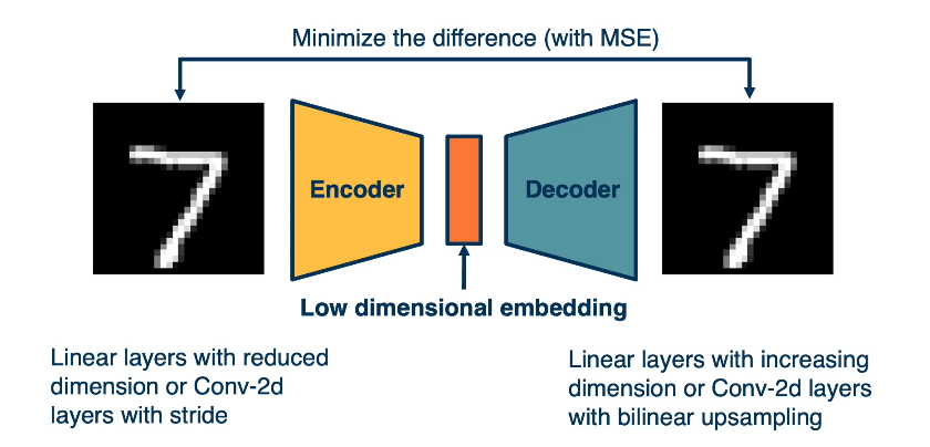
We know what the input is, we want to reconstruct it, we don’t need any labels. And this also allows us to use a very concrete loss function, that is we can minimize the difference with mean squared error for example, between the input and the reconstructed input.

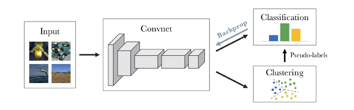
Another thing we can leverage is the clustering assumption. This is common in unsupervised learning, where we assume that high density regions form clusters, that is items or instances that are similar form groups or clumps in some feature space. While low density region, that is regions where there’s not a lot of examples separate clusters, which hold semantic meaning.

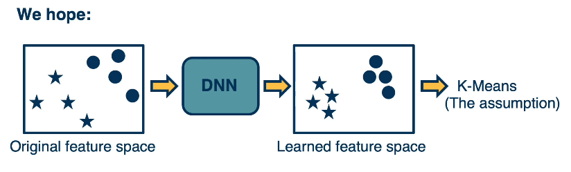
The key idea is that whatever feature space we learned, we’d like those feature spaces to have these kinds of characteristics. We’d like them to essentially have features that are similar to similar items and features that are far apart, according to some distance metric or elements that are different. And so, this is what we’re hoping, we’re hoping that essentially whatever original feature space or raw input space we feed.Once we’ve output feature space that’s transformed using a deep neural network, we’d like that feature space to have this property. One thing that we can test this property with is apply K-Mean.

While a lot of these tasks have already existed before deep learning, for example, reconstruction is an optimization criteria for principal component analysis. And clustering has long existed before deep learning, we can actually generalize this idea into the concept of surrogate tasks. That is we’d like to come up with tasks where we can get the answer or label for free in order to drive optimization and prevent the need for human annotation. These tasks though, must also force the neural network to learn effective feature representation. And we’d like to engineer the tasks so that there aren’t any trivial solutions or ways that the neural network can cheat to prevent it from learning effective feature representation. It turns out that over the years, a large number of such tasks have been devised, and they all have different characteristics in terms of how effective the features that are learned are. And this can differ both in terms of the level at which the neural network learns features.

For example, low-level edge features versus high-level semantic features, as well as how well they can generalize to other tasks as well. One example is colorization. Given a red, green, blue three channel image, we can actually just convert it to grayscale. This can be done using a hard coded formula. And the input to a neural network will then be this grayscale image. And we’d like it to re-colorize the image. Now clearly, this forces the neural network to have to understand something about what is in the image. Otherwise it’s really hard to colorize. For example, if you don’t know that this is a fish or what type of fish it is or if you have other objects such as tennis balls and so on, it’s going to be really hard to apply the same color. And what’s nice is that we know the answer, we already have the original RGB image. So we can have the neural network predicts the colorized image and we can use for example, a mean squared error loss function to drive feature learning.

There’s a specific way that we evaluate the results of these surrogate tasks. Specifically, what we’d like to do is answer the question how good are the feature representations that we learn in an unsupervised manner and how well do they generalize to new label tasks. And so what we typically do is just take the encoder part, for example in the rotation prediction, we don’t actually care about the layer that actually predicts the rotation amount. And then we transfer it to the actual task. This is essentially transfer learning where we use it to initialize the model of another supervised learning task. And we really use what we learned in an unsupervised way to extract features such that we can add another classifier on top, typically a neural network or prior machine learning methods such as support vector machines. Often we limit the classifier to simple linear layers. This is because we’re interested in how good are the feature representations that we learn and how generalizable are they. So if we’re comparing many different surrogate tasks with each other, we don’t wanna have another confounding effect by adding additional complex transformations or nonlinearity. That wouldn’t essentially tell us how good or the feature representations, but it kind of adds the additional element of training those additional layers. So typically we just take the features from the unsupervised surrogate tasks and then add a linear layer to whatever supervised classification task we’d like.

In summary, there’s a large number of surrogate tasks and variations that we can use to learn really good feature representations using unlabeled data alone. This includes contrast of losses which work across image patches or context or instance discrimination. And there’s many different types of loss functions or training regimes that we can apply some of them more efficient than others. The two that have become dominant and extremely effective are for unsupervised learning. Contrastive losses and when we have semi supervised learning, pseudo labeling losses, where we have essentially the learned model applied to the labeled data, making predictions on the unlabeled data and that gets used to drive a cross entropy loss. You can also use soft knowledge distillation where you don’t make the prediction of one hot for the pseudo-label. And I haven’t covered all of these methods but a lot of these methods work and it’s not clear which one is the best currently. What we do know is that data augmentation is now key. These methods are used across almost all of these unsupervised learning and semi-supervised learning methods. And maybe unfortunately, methods tend to be sensitive to the choice of data augmentation. So there’s a lot of recent work exploring how we can automatically learn data augmentation or be able to figure out at least, what data augmentation to use. Overall, these advances have been extremely exciting and have really only occurred recently.