Learning Objectives
- Reinforcement Learning
- Markov Decision Processes
- Algorithms for solving MDPs
- DQN: Deep Q-Learning
- Policy Gradients, Actor Critic
In this module, we’ll talk about advanced topics, that is we’ll show the power of deep learning and moving beyond just the standard supervised machine learning setting that we’ve talked about thus far. For example, we’ll try to address the problem of how to deal with unlabeled data, which is much easier to collect. And where we don’t have a lot of labeled data, that is annotations that humans have made or given for each piece of data that we have. We’ll also try to cover decision making tasks, which moves beyond just making predictions on pieces of data. But actually allows the neural network to make the decisions in the form of actions that actually affect the world.
Reinforcement Learning
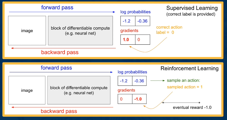
In this section, we will introduce reinforcement learning where the task is to make a sequence of decisions or predictions similar to what you’re seeing in sequence models. However, we will not receive supervision in the form of the correct decision or a prediction which should have been made. Instead, we will only receive evaluative feedback in the form of reward for the decision or our prediction which was made.
Definition Reinforcement learning can be defined in one sentence as a sequential decision, making in an environment with evaluative feedback.
Let’s break the last sentence into it’s component parts.
Environment
Let’s break this definition down by first talking about what we mean by an environment. For that, let’s imagine we have an agent who can take actions in an environment and the environment produces a state which the agent can persist. In addition to giving a reward to the agent for the actions it did take. Now this environment may be unknown, very complex.
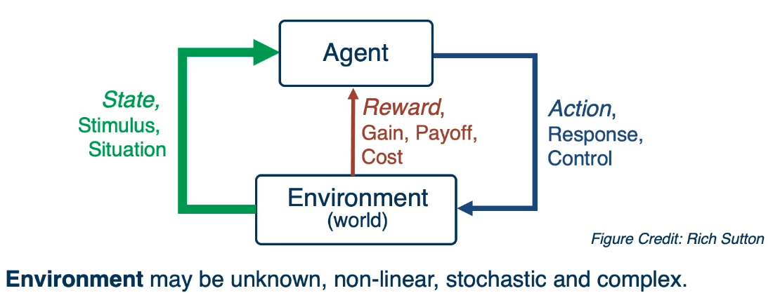
Think of the worst case as a real robot being deployed in the world, in which case the environment is the real world. The task of this agent is to learn a policy to map states of the environment to actions that it can play to affect the environment. The objective of this agent is to maximize the reward it will get from the environment in the long run.
Evaluative feedback
Evaluative feedback means that the agent is supposed to pick actions and receive rewards which can be positive or negative only for the actions that it did take and not for the actions that did not take. This means that the agent will never know or have supervision for the correct or best action that it should have taken at a particular state.
Sequential decisions
Unlike supervised learning, and sequential decisions just means that the agent needs to make a sequence of actions or a sequence of states in order to complete the task. And with this what can happen is that the reward may be delayed and it can only happen at the end of the task, which means that the agent needs to optimize in the long term for rewards it may get at a very very later stage.
Challenges
- To evaluate a feedback implies that the best action can only be found through trial and error, requiring the agent to try all possible actions at all states.
- In order to be 100% certain about the best action, the agent may not receive reward for every action it takes, requiring long term planning in order to eventually get high rewards in the future.
- Updates made to the policy during learning will lead to changes in the actions that are picked by the policy and hence will change the data distribution of states and rewards that the policy absorbs making this distribution non stationary.
- Further, if the task involves streaming data, the agent will see certain states only once and never again in his lifetime, making it difficult to learn from past mistakes.
The protocol for how the agent interacts with the environment
- At every time step t
++ the agent will receive an observation $o_t$
++ it will execute an action $a_t$
- In the environment at time step t
++ the environment will receive this action $a_t$
++ and produce a new observation $o_{t+1}$, as well as a reward $r_{t+1}$
- RL has also been applied to games like GO where the objective is to defeat the opponent.
++ The state of the environment is the location of the pieces on the board.
++ The action is where to put down the next piece and
++ The reward in this case is quite sparse.
It is plus one for winning the game or zero otherwise, making it an exceptionally challenging long term planning task.
Markov Decision Processes
Markov decision processes, MDPs, form the underlying framework of Reinforcement learning. They can be defined as a tuple of five values:
- S - The set of all possible states of the environment
- A - The set of all possible actions that can be taken at every step
- R(s,a,s’) - Is the reward distribution given a state S, action A, and next state S′
- T(s,a,s’) - is the transition probability distribution, of the next state S’
- often written as p(s’|s,a)
- γ- is the discount factorS - The set of all possible states of the environment
We can now define an Interaction Trajectory as a sequence of state/action/rewards
Markov Property
The Markov processes are an important class of the stochastic processes. The Markov property means that evolution of the Markov process in the future depends only on the present state and does not depend on past history. The Markov process does not remember the past if the present state is given. Hence, the Markov process is called the process with memoryless property.
MDPs are characterized by the Markov property, which as seen by the definition of the transition probability. It implies that the distribution of possible next states given state s, and action a, Does not depend on any of the previous states or actions in the trajectory.
In Reinforcement learning, we assume an underlying MDP with unknown Transition probability distribution T and Reward distribution R
Instead, only samples from these distributions are observed by the agent interacting with the environment. Evaluative feedback comes into play, because of the lack of knowledge in the reward distribution. This will require a trial and error approach to determine rewards.
For our discussions we will assume known reward and transition functions. This will allow us to look at algorithms for solving MDPs, which comes down to finding the best policy. Which can be loosly defined as the best action for each possible state s in the set of all possible states
- Rewards are known everywhere, no evaluative feedback
- Know how the world works, ie all transitions
Let’s take a look at a simple environment, (see below), where we can intuitively figure out what is the best policy. The 2D environment below is a grid world, where there’s an agent indicated by a blue triangle. Where the state of the environment is the 2D coordinates of this agent. In which case the agent right now is at (2,3). The actions that the agent can take is either move one cell north, east, south, or west. And the rewards are either +1 or -1 at the absorbing states shown in the figure on the right.
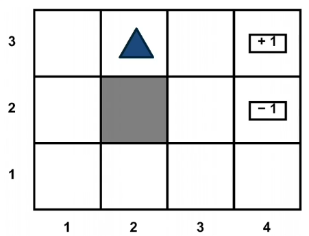
With this setup, it is easy to see that the optimal policy is to head east twice, in order to reach the +1 absorbing state. However, let’s assume that there is some noise in how the agent transitions to next state. This noise is in the form of a 20% chance, of the agent drifting once a left or right of the direction of motion. Now, things get a bit complicated. The policy will now have to prescribe an action, for the states that the agent could land up in. As it is not guaranteed to always move in the direction of east. One way to describe such a policy, would be in the form of a 2D matrix, of the same shape as this 2D grid. But each matrix element is prescribing an action to take, if the agent is at that cell. This leads us to the formal definition of a policy, that we will use for solving MDPs.
Formally a policy is a mapping from states to actions
Deterministic Policy : $\pi(s)=a$
Stochastic Policy : $\pi(a|s)=P(A_t=a|S_t=s)$
What defines a good policy?
- Maximize current rewards vs Sum of all rewards where γ∈[0,1]
- Discounted sum of future rewards!
- Now 1, next step γ, 2 steps from now γ2
We can now define the optimal policy as
$$\pi^∗=argmax_πE[\sum_{t≥0}γ^tr_t|π]$$
Expected Value here is taken over
- Initial State $s_0∼p(s_0)$
- Actions from policy $a_t∼π(⋅|s_t)$
- Next States $s_{t+1}∼p(⋅|s_t,a_t)$ from the transition distribution
Note the discount term raised to the power of t. This implies that immediate rewards are preferred over future rewards.
We need to now introduce one last component the value function. The value function is a prediction of discounted sum of future rewards.
- State value function, V-function, V:S→R
- maps the state to real values
- This allows us to measure the “goodness” of a state
- State-Action value function, Q-Function Q:S×A→R
- This allows us to measure the goodness of the state-action pair
- It will also tell us the impact of this action on the future
For a policy that produces a trajectory sample $(s_0,a_0,s_1,a_1,⋯)$
The V-function of the policy at state s, is the expected discounted sum of rewards from state s:
$$V^π(s)=E[\sum_{t≥0}γ^tr_t|π,s_0=s]$$
The Q-Function of the policy at state s and action a is the expected cumulative reward upon taking action a in state s (and following policy thereafter):
$$Q^π(s,a)=E[\sum_{t≥0}γ^tr_t|π,s_0=s,a_0=a]$$
Algorithms for Solving MDPs
Optimal V & Q functions
In the previous section, see above, we defined the V and Q functions for all policies π. In a simple slight of hand you can define the Q and V for the optimal policy by simply using the * notation to denote the optimal policy.
ie
$$V^∗(s)=E[\sum_{t≥0}γ^tr_t|π^*,s_0=s]$$
Similarly
$$Q^∗(s,a)=E[\sum_{t≥0}γ^tr_t|π^*,s_0=s,a_0=a]$$
Now these two equation are highly interconnected, via the optimal, and have the following identities, with subtle yet important difference in interpretation
$$V^∗(s)=max_aQ^∗(s,a)$$
- it says that the optimal value at a state is the same as the max Q value over all possible actions at that state
$$\pi^∗(s)=argmax_aQ^∗(s,a)$$
- it says that the optimal policy at state s will occur at the action a that maximizes the Q function at that state
Taking a closer look at the definition of the optimal Q function, we will now try to rewrite it recursively in terms of the optimal value function at future states. Let’s define the term return as the sum of discounted future rewards.
Bellman Optimality Equations
Taking a closer look at the definition of the optimal Q function, we will now try to rewrite it recursively in terms of the optimal value function at future states. Let’s define the term return as the sum of discounted future rewards.
At time step t=0 our expected return is
$$Q^∗(s,a)=E[\sum_{t≥0}γ^tr(s,a)|s_0=s,a_0=a]$$
Where the expected value is taken over $a_t∼π^∗(⋅|s_t)$ and $s_{t+1}∼p(⋅|s_t,a_t)$
If we look ahead to time step t=1, we get (a reward from t=0) + (the discounted return from t=1)
$$
\large = \gamma^0 r(s,a) + \mathbb{E}{s’ \sim p(\cdot | s,a)}
\left[ \gamma \mathbb{E}{a_t \sim \pi^*(\cdot|s_t) \text{ and } s_{t+1}\sim p(\cdot|s_t,a_t)}
[ \sum_{t \geq 1} \gamma^{t-1} r(s_t,a_t) | s_1 = s’ ] \right]
$$
( Now imagine the next few steps because typing these equations in Latex is rather tedious)
We can now use this to put together to derive the bellman optimality equations
$$Q^∗(s,a)=E_{s′∼p}(s’|s,a)[r(s,a)+γV^∗(s′)]\\
=\sum_{s′}p(s′|s,a)[r(s,a)+γV^∗(s′)]\\
=\sum_{s′}p(s′|s,a)[r(s,a)+γmaxa′Q^∗(s′,a′)]$$
Similarly we can also define $V^∗$ as follows
$$V^∗(s)=max_a\sum_{s′}p(s′|s,a)[r(s,a)+γV^∗(s′)]$$
Value-Iteration
And we can use it to define an algorithm as follows
- Initialize values of all states
- While not converged
- For each state
- $V^{i+1}(s)←max_a\sum_{s′}p(s′|s,a)[r(s,a)+γV^∗(s′)]$
- Repeat until convergence (no change in values)
- $V^0→V^1→⋯→V^i→⋯→V^∗$
Q-Iteration
Intuitively, each application of this recursive equation can be thought of as propagating the information of the return at a state s to the return values of its neighboring states under the transition probability. This update will produce a sequence of vectors V0, V1, and so on, until we get V star upon convergence.
Given the nature of the upgrade step, each iteration of this algorithm will have a time complexity order $O(S^2A)$, where S is the cardinality of the state space and A is the cardinality of the action space.
In a similar fashion we can derive the Q function recursively as follows
$$
\large Q^{i+1}(s,a) = max_a \sum_{s’} p(s’|s,a) [r(s,a) + \gamma \color{red}{max_{a’} Q^i(s’,a’)} ]
$$
Which is basically the same as before, except for the last loop over the actions to get max a.
So all this begs the question of how to determine the optimal policy??
Pollicy Iteration
Begin with $π_0$ and iteratively refine it: $π_0→π_1→⋯→π_i→⋯→π^∗$
Involves repeating two steps:
- Policy Evaluation: Compute $V^π$ similar to Value Iteration
- Policy Refinement: Greedily change actions as per $V^π$ at next states
- $\color{red}{\pi_{i}(s)} \leftarrow argmax_a \sum_{s’} p(s’|s,a) [r(s,a) + \gamma \color{red}{V^{\pi_i}(s’)} ]$
$π_i$ may seem a bit out of place but it turns out that it converges to π∗ much faster than V^{πi} does to V^{π∗}
Another possible algorithm is Value Iteration. which we leave to the reader to research
DQN: Deep Q-Learning
Deep Q-learning assumes a parametrized Q-function that is optimised to match the optimal Q-function, from a defined data set of state, action, next state and reward tuples as shown below. The simplest example of such a parameters network, is a linear Q-network with one weight vector and a bias. Alternatively, the Q-network can also be a deep neural network.
Intuition: to learn a parametrized Q-Function from data ${ (s,a,s’,r)i }{i=1}^N$
Examples:
- A simple/basic example of such a function is Q-Learning with linear function approximators
- $Q(s,a;w,b) = W_a^T s + b_a$
- Another example is Deep Q Learning by fitting a Q-Network
- $Q(s,a;\theta)$
- works well in practice
- Q Network can take RGB images
CASE Study
- this was used to develop a Q learning network that could play atari games. It used the last 4 images to represent the state
Updating the Q function is the application of the bellman equation seen before
$$\color{red}{Q^*(s,a)} = \mathbb{E}{s’ \sim p(s’|s,a)} [r(s,a) + \gamma \color{blue}{max{a’} Q^*(s’,a’)}]$$
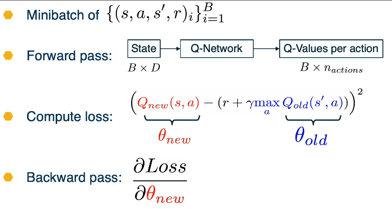
During training, we can use a single Q-network to predict the Q-values for the current state and action shown on the left, and the next state and next actions shown in blue on the right. Instead of having a for loop over all states to update the Q-network, as was done in Q-iteration, we introduced a regression objective that will minimize this mean squared error.
Loss for a single point
- MSE Loss := $\color{red}{Q_{new}(s,a)} - (r + \gamma \color{blue}{max_{a’} Q_{old}(s’,a’)})^2$
- Where $Q_{new}$ is the predicted value
- and $(r + \gamma \color{blue}{max_{a’} Q_{old}(s’,a’)})$ is the target Q-Value
Intuitively, this will attempt to make the predicted Q-values in red, match the target Q-values on the right. However, in practice, it has been observed that using a single Q-network, makes the loss minimization unstable.
For stability purposes you can
- Freeze $Q_{old}$ and update $Q_{new}$ parameters
- ie Set $Q_{old}←Q_{new}$ at regular intervals
Assuming a fixed dataset, the Avg MSE Loss can be optimized using the Fitted Q-Iteration Algorithm. However, the question is how to gather experience or “data”? This is why RL is hard!
There are two challenges:
Challenge 1: Exploration vs Exploitation
- Exploration refers to the process of the agent trying out different actions in the environment to gain more information about the potential rewards associated with different states and actions.
- Exploitation, on the other hand, involves the agent choosing actions that are believed to be the best based on its current knowledge or Q-value estimates.
Challenge 2: Non iid, highly correlated data
High Level look at gathering data
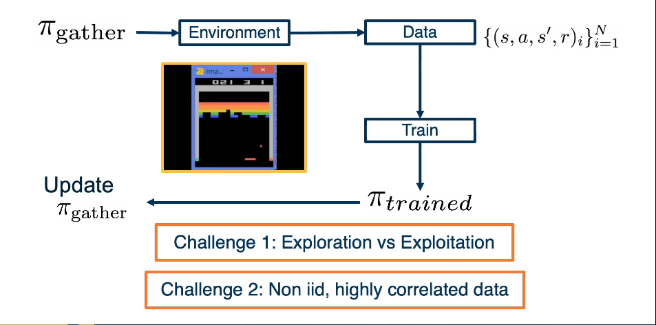
What should $\pi_{gather}$ be?
Greedy? => Local minimas, no exploration
- argmaxaQ(s,a;θ)
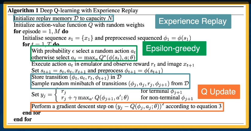
- ϵ greedy exploration strategy
- $a_t=argmax_aQ(s,a)$ with probability 1−ϵ
- or $a_t=random$ action with probability ϵ
It should be noted though that there are potentially large pitfalls in this approach. If samples are correlated, then this leads to high variance gradients, which leads to inefficient learning.
This can be remedied by experience replay.
- A replay buffer stores transitions (s,a,s′,r)
- Continually update replay buffer as game (experience) epsiodes are played, older are samples discarded
- Train Q-Network on random minibatches of transitions from replay memory, instead of consecutive samples
- The larger the buffer the lower the correlation
Now that we have all the needed pieces, we can fully understand and implement the original Deep Q-Learning Alogrithm
Policy Gradients, Actor Critic
In this lecture, we will study a family of policy based RL Algorithms, which are based on graded updates or paramterized policies.
Among the types of methods used in RL are
- value based methods to learn Q-functions
- model based methods to learn transition and reward functions.
However, both methods provide an optimal policy that is used to perform a task with a high reward.
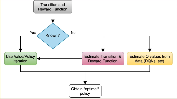
Policy based methods on the other hand directly parameterize a policy and optimize it to maximize returns.
Our class of Policies is parametrized by the family of parameters given by θ, which can be the parameters of a linear transformation, or deep network, or other possibilities.
Formally
- $\large \pi_{\theta}(s|a) : \mathcal{S} \rightarrow \mathcal{A}$
- The objective function we want to maximize is given by
- $\large J(\pi) = \mathbb{E}[\sum_{t=1}^T \mathcal{R}(s_t,a_t)]$
- we assume γ=1 for this discussion
Going forward we will adjust our notation to properly convey our goal
- Our original optimal policy was defined as
- $\pi^* = \text{argmax}{\pi:\mathcal{S} \rightarrow \mathcal{A}} \mathbb{E}[\sum{t=1}^T R(s_t,a_t)]$
- Our new way
- \theta^* = \text{argmax}{\theta} \mathbb{E}[\sum{t=1}^T R(s_t,a_t)]
To be clear this is not a change in the definition. It’s simply making explicit that the optimal parameters fully describe the optimal policy
Let’s now do a walkthrough of a policy based algorithm
Step 1: Data Gathering
We begin by defining a finite trajectory tau as
$$\tau = (s_0,a_0,\cdots,s_T,a_T)$$
The probability of tau given a policy $\pi_\theta$, is denoted $\pi_\theta(\tau)$, is given by
$$
\begin{split}
\pi_{\theta}(\tau) & = p_{\theta}(\tau) \
& = p_{\theta}(s_0,a_0,\cdots,s_T,a_T) \
& = p(s_0) \prod_{t=0}^T p_{\theta}(a_t|s_t) \cdot p(s_{t+1}|s_t,a_t)
\end{split}
$$
Further, we will write our objective as finding the parameters theta that maximizes the expected sum of rewards over trajectories tau.
$$\large \text{argmax}{\theta} \mathbb{E}{\tau \sim p_{\theta}(\tau)} [\mathcal{R}(\tau)]$$
Now we can gather data in a much simpler form than before
- We already have a policy $\tau_\theta$
- So we can Sample N trajectories ${\tau i}^N_{i=1}$ by acting according to $\pi_\theta$
- this is a small batch of trajectories using the current $\pi_\theta$, which can be used as a sample based approximation of our reward objective.
In the next few slides, when we formally derive our policy gradient expression, we will see a similar expectation that will again use the same batch of trajectories to estimate the gradient update.
$$\approx \frac{1}{N} \sum_{i=1}^N \sum_{t=1}^T r(s_t^i, a_t^i)$$
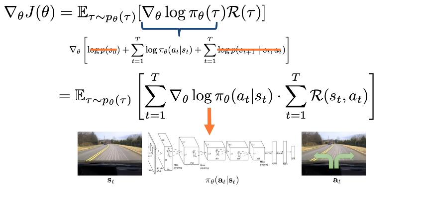
Let’s now derive the policy gradient
$$
\large
\begin{split}
\nabla_{\theta} J(\theta) & = \nabla_{\theta} \mathbb{E}{\tau \sim p{\theta}}(\tau) [\mathcal{R}(t)] \
& = \nabla_{\theta} \int \pi_{\theta}(\tau) \mathcal{R}(\tau) d\tau \
& = \int \nabla_{\theta} \pi_{\theta}(\tau) \mathcal{R}(\tau) d\tau \
& = \int \nabla_{\theta} \pi_{\theta}(\tau) (\frac{\pi_{\theta}(\tau)}{\pi_{\theta}(\tau)}) \mathcal{R}(\tau) d\tau \
& = \int \pi_{\theta}(\tau) \nabla_{\theta} \text{log}\pi_{\theta}(\tau) \mathcal{R}(\tau) d\tau \
& = \mathbb{E}{\tau \sim p{\theta}}(\tau) [\nabla_{\theta} \text{log}\pi_{\theta}(\tau) \mathcal{R}(\tau)]
\end{split}
$$
Note that we used the identity
$$\large \nabla_{\theta} \text{log}\pi_{\theta}(\tau) = (\frac{\nabla_{\theta} \pi_{\theta}(\tau)}{\pi_{\theta}(\tau)})$$
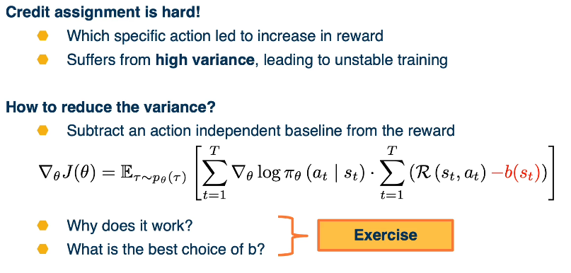
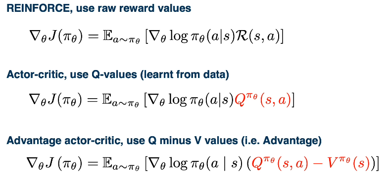
The key idea behind these variations is that subtracting some baseline b shown in red, that does not depend on actions will preserve the mean of the gradient expectation while possibly reducing the variance for specific choices of B. The proof of why the mean is not affected by such a baseline. And what is the best choice of such a baseline is left as an exercise. The different choices of this baseline have resulted in two important variants of the policy gradient algorithm. The first is known as the actor-critic algorithm that replaces rewards with the Q function of the policy that is learned from data. The second algorithm is known as advantage actor-critic that substitutes the reward with the advantage of the policy. It is defined as the Q function minus the V function.