Learning Objectives
- Various sequence to sequence architectures
- Speech recognition - Audio data
Sequence models can be augmented using an attention mechanism. This algorithm will help your model understand where it should focus its attention given a sequence of inputs. Here, you will also learn about speech recognition and how to deal with audio data.
Various sequence to sequence architectures
Basic Models
Sequence-to-sequence models are useful for everything from machine translation to speech recognition.
Machine translation
Papers:
- Sequence to Sequence Learning with Neural Networks by Ilya Sutskever, Oriol Vinyals, Quoc V. Le.
- Learning Phrase Representations using RNN Encoder-Decoder for Statistical Machine Translation by Kyunghyun Cho, Bart van Merrienboer, Caglar Gulcehre, Dzmitry Bahdanau, Fethi Bougares, Holger Schwenk, Yoshua Bengio.
Input a French sentence: Jane visite l’Afrique en septembre, we want to translate it to the English sentence: Jane is visiting Africa in September.
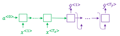
- First, let’s have a network, which we’re going to call the encoder network be built as a RNN, and this could be a GRU and LSTM, feed in the input French words one word at a time. And after ingesting the input sequence, the RNN then offers a vector that represents the input sentence.
- After that, you can build a decoder network which takes as input the encoding and then can be trained to output the translation one word at a time until eventually it outputs the end of sequence.
- The model simply uses an encoder network to find an encoding of the input French sentence and then use a decoder network to then generate the corresponding English translation.

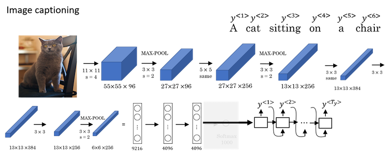
Image Captioning
- This architecture is very similar to the one of machine translation.
- Paper: Deep Captioning with Multimodal Recurrent Neural Networks (m-RNN) by Junhua Mao, Wei Xu, Yi Yang, Jiang Wang, Zhiheng Huang, Alan Yuille.
- In previous course, you’ve seen how you can input an image into a convolutional network, maybe a pre-trained AlexNet, and have that learn an encoding or learn a set of features of the input image.
- In the AlexNet architecture, if we get rid of this final Softmax unit, the pre-trained AlexNet can give you a 4096-dimensional feature vector of which to represent this picture of a cat. And so this pre-trained network can be the encoder network for the image and you now have a 4096-dimensional vector that represents the image. You can then take this and feed it to an RNN, whose job it is to generate the caption one word at a time.
Picking the most likely sentence
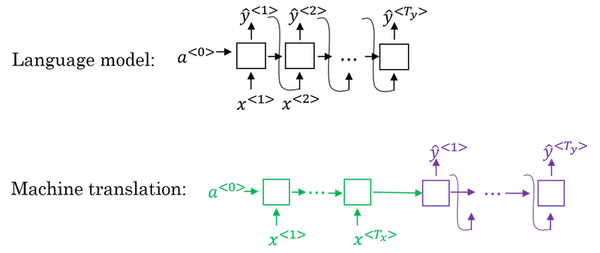
There are some similarities between the sequence to sequence machine translation model and the language models that you have worked within the first section of this course, but there are some significant differences as well.
The machine translation is very similar to a conditional language model.
- You can use a language model to estimate the probability of a sentence.
- The decoder network of the machine translation model looks pretty much identical to the language model, except that instead of always starting along with the vector of all zeros, it has an encoder network that figures out some representation for the input sentence.
- Instead of modeling the probability of any sentence, it is now modeling the probability of the output English translation conditioned on some input French sentence. In other words, you’re trying to estimate the probability of an English translation.
- The difference between machine translation and the earlier language model problem is: rather than wanting to generate a sentence at random, you may want to try to find the most likely English translation.
- In developing a machine translation system, one of the things you need to do is come up with an algorithm that can actually find the value of y that maximizes
p(y<1>,...,y<T_y>|x<1>,...,x<T_x>). The most common algorithm for doing this is called beam search.- The set of all English sentences of a certain length is too large to exhaustively enumerate. The total number of combinations of words in the English sentence is exponentially larger. So it turns out that the greedy approach, where you just pick the best first word, and then, after having picked the best first word, try to pick the best second word, and then, after that, try to pick the best third word, that approach doesn’t really work.
- The most common thing to do is use an approximate search out of them. And, what an approximate search algorithm does, is it will try, it won’t always succeed, but it will to pick the sentence, y, that maximizes that conditional probability.
Beam Search
In the example of the French sentence, "Jane, visite l'Afrique en Septembre".
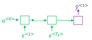
Step 1: pick the first word of the English translation.
- Set beam
width B = 3. - Choose the most likely three possibilities for the first words in the English outputs. Then Beam search will store away in computer memory that it wants to try all of three of these words.
- Run the input French sentence through the encoder network and then this first step will then decode the network, this is a softmax output overall 10,000 possibilities (if we have a vocabulary of 10,000 words). Then you would take those 10,000 possible outputs p(y<1>|x) and keep in memory which were the top three.
- For example, after this step, we have the three words as in,
Jane, September.
- Set beam
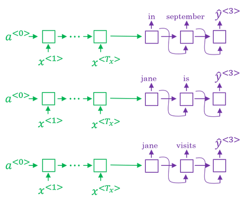
Step 2: consider the next word.
- Find the pair of the first and second words that is most likely it’s not just a second where is most likely. By the rules of conditional probability, it’s p(y<1>,y<2>|x) = p(y<1>|x) * p(y<2>|x,y<1>).
- After this step,
in september, jane is, jane visitis left. And notice thatSeptemberhas been rejected as a candidate for the first word. - Because
beam widthis equal to 3, every step you instantiate three copies of the network to evaluate these partial sentence fragments and the output. - Repeat this step until terminated by the end of sentence symbol.
- If beam width is 1, this essentially becomes the greedy search algorithm.
Refinements to Beam Search
Length normalization:
Beam search is to maximize the probability:

But multiplying a lot of numbers less than 1 will result in a very tiny number, which can result in numerical underflow.
So instead, we maximizing a log version:

If you have a very long sentence, the probability of that sentence is going to be low, because you’re multiplying many terms less than 1. And so the objective function (the original version as well as the log version) has an undesirable effect, that maybe it unnaturally tends to prefer very short translations. It tends to prefer very short outputs.
A normalized log-likelihood objective:
- 𝛼 is another hyperparameter
- 𝛼=0 no normalizing
- 𝛼=1 full normalization
How to choose beam width B?
- If beam width is large:
- consider a lot of possibilities, so better result
- consuming a lot of different options, so slower and memory requirements higher
- If beam width is small:
- worse result
- faster, memory requirements lower
- choice of beam width is application dependent and domain dependent
- In practice, B=10 is common in a production system, whereas B=100 is uncommon.
- B=1000 or B=3000 is not uncommon for research systems.
- But when B gets very large, there is often diminishing returns.
Unlike exact search algorithms like BFS (Breadth First Search) or DFS (Depth First Search), Beam Search runs faster but is not guaranteed to find exact maximum for $argmax_y𝑃(𝑦|𝑥)$.
Error analysis in beam search
- Beam search is an approximate search algorithm, also called a heuristic search algorithm. And so it doesn’t always output the most likely sentence.
- In order to know whether it is the beam search algorithm that’s causing problems and worth spending time on, or whether it might be the RNN model that’s causing problems and worth spending time on, we need to do error analysis with beam search.
- Getting more training data or increasing the beam width might not get you to the level of performance you want.
- You should break the problem down and figure out what’s actually a good use of your time.
- The error analysis process:
Problem:
- To translate:
Jane visite l’Afrique en septembre.(x) - Human:
Jane visits Africa in September.(y*) - Algorithm:
Jane visited Africa last September.(ŷ) which has some error.
- To translate:
Analysis:
- Case 1:
Human Algorithm p(y*|x) vs p(ŷ|x) At fault? Jane visits Africa in September. Jane visited Africa last September. p(y*|x) > p(ŷ|x) Beam search … … … … - Case 2:
Human Algorithm p(y*|x) vs p(ŷ|x) At fault? Jane visits Africa in September. Jane visited Africa last September. p(y*|x) ≤ p(ŷ|x) RNN … … … …
Attention Model Intuition
Paper: Neural Machine Translation by Jointly Learning to Align and Translate by Dzmitry Bahdanau, Kyunghyun Cho, Yoshua Bengio.
You’ve been using an Encoder-Decoder architecture for machine translation. Where one RNN reads in a sentence and then different one outputs a sentence. There’s a modification to this called the Attention Model that makes all this work much better.
The French sentence:
Jane s'est rendue en Afrique en septembre dernier, a apprécié la culture et a rencontré beaucoup de gens merveilleux; elle est revenue en parlant comment son voyage était merveilleux, et elle me tente d'y aller aussi.
The English translation:
Jane went to Africa last September, and enjoyed the culture and met many wonderful people; she came back raving about how wonderful her trip was, and is tempting me to go too.
The way a human translator would translate this sentence is not to first read the whole French sentence and then memorize the whole thing and then regurgitate an English sentence from scratch. Instead, what the human translator would do is read the first part of it, maybe generate part of the translation, look at the second part, generate a few more words, look at a few more words, generate a few more words and so on.
The Encoder-Decoder architecture above is that it works quite well for short sentences, so we might achieve a relatively high Bleu score, but for very long sentences, maybe longer than 30 or 40 words, the performance comes down. (The blue line)
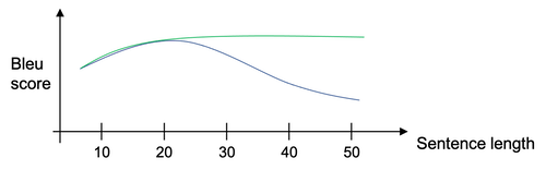
The Attention model which translates maybe a bit more like humans looking at part of the sentence at a time. With an Attention model, machine translation systems performance can look like the green line above.
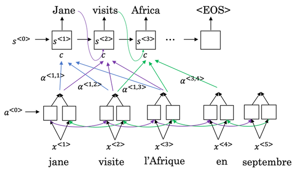
What the Attention Model would be computing is a set of attention weights and we’re going to use
𝛼<1,1>to denote when you’re generating the first words, how much should you be paying attention to this first piece of information here and𝛼<1,2>which tells us what we’re trying to compute the first word of Jane, how much attention we’re paying to the second word from the inputs, and𝛼<1,3>and so on.Together this will be exactly the context from, denoted as C, that we should be paying attention to, and that is input to the RNN unit to try to generate the first word.
In this way the RNN marches forward generating one word at a time, until eventually it generates maybe the
<EOS>and at every step, there are attention weighs𝛼<t,t'>that tells it, when you’re trying to generate the t-th English word, how much should you be paying attention to the t’-th French word.
Attention Model
Assume you have an input sentence and you use a bidirectional RNN, or bidirectional GRU, or bidirectional LSTM to compute features on every word. In practice, GRUs and LSTMs are often used for this, maybe LSTMs be more common. The notation for the Attention model is shown below.
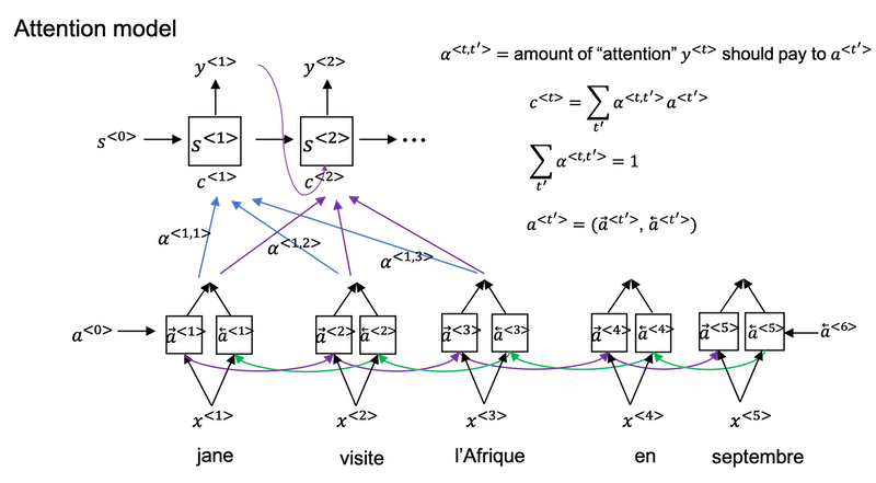
Compute attention weights:

Compute
e<t,t'>using a small neural network:- And the intuition is, if you want to decide how much attention to pay to the activation of t’, it seems like it should depend the most on is what is your own hidden state activation from the previous time step. And then
a<t'>, the features from time step t’, is the other input. - So it seems pretty natural that
𝛼<t,t'>ande<t,t'>should depend ons<t-1>anda<t'>. But we don’t know what the function is. So one thing you could do is just train a very small neural network to learn whatever this function should be. And trust the backpropagation and trust gradient descent to learn the right function.
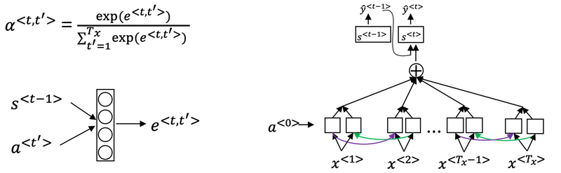
- And the intuition is, if you want to decide how much attention to pay to the activation of t’, it seems like it should depend the most on is what is your own hidden state activation from the previous time step. And then
One downside to this algorithm is that it does take quadratic time or quadratic cost to run this algorithm. If you have $T_x$ words in the input and $T_y$ words in the output then the total number of these attention parameters are going to be $T_x \times T_y$.
Visualize the attention weights
𝛼<t,t'>: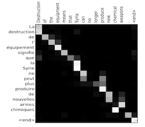
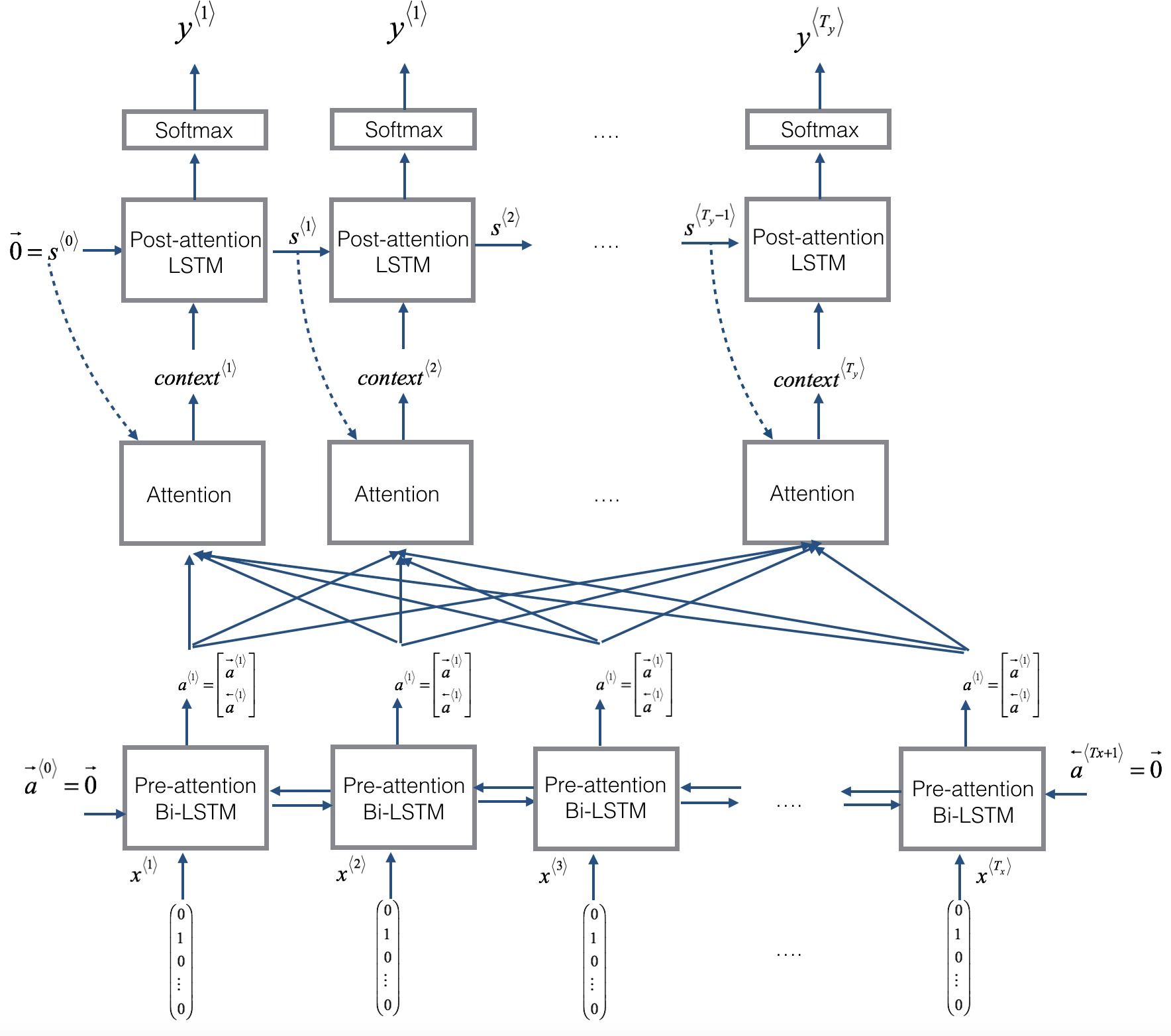
Implementation tips:
- The diagram on the left shows the attention model.
- The diagram on the right shows what one “attention” step does to calculate the attention variables
𝛼<t,t'>. - The attention variables
𝛼<t,t'>are used to compute the context variablecontext<t>for each timestep in the output (t=1, …, Ty).
Speech recognition - Audio data
Speech recognition
- What is the speech recognition problem? You’re given an audio clip, x, and your job is to automatically find a text transcript, y.
- So, one of the most exciting trends in speech recognition is that, once upon a time, speech recognition systems used to be built using phonemes and this were, I want to say, hand-engineered basic units of cells.
- Linguists use to hypothesize that writing down audio in terms of these basic units of sound called phonemes would be the best way to do speech recognition.
- But with end-to-end deep learning, we’re finding that phonemes representations are no longer necessary. But instead, you can built systems that input an audio clip and directly output a transcript without needing to use hand-engineered representations like these.
- One of the things that made this possible was going to much larger data sets.
- Academic data sets on speech recognition might be as a 300 hours, and in academia, 3000 hour data sets of transcribed audio would be considered reasonable size.
- But, the best commercial systems are now trains on over 10,000 hours and sometimes over a 100,000 hours of audio.
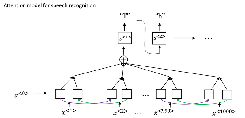
How to build a speech recognition?
- Attention model for speech recognition: one thing you could do is actually do that, where on the horizontal axis, you take in different time frames of the audio input, and then you have an attention model try to output the transcript like, “the quick brown fox”.
CTC cost for speech recognition: Connectionist Temporal Classification
Paper: Connectionist Temporal Classification: Labelling Unsegmented Sequence Data with Recurrent Neural Networks by Alex Graves, Santiago Fernandes, Faustino Gomez, and Jürgen Schmidhuber.

For simplicity, this is a simple of what uni-directional for the RNN, but in practice, this will usually be a bidirectional LSTM and bidirectional GRU and usually, a deeper model. But notice that the number of time steps here is very large and in speech recognition, usually the number of input time steps is much bigger than the number of output time steps.
- For example, if you have 10 seconds of audio and your features come at a 100 hertz so 100 samples per second, then a 10 second audio clip would end up with a thousand inputs. But your output might not have a thousand alphabets, might not have a thousand characters.
The CTC cost function allows the RNN to generate an output like
ttt_h_eee___[]___qqq__, here_is for “blank”,[]for “space”.The basic rule for the CTC cost function is to collapse repeated characters not separated by “blank”.
Trigger Word Detection
- With the rise of speech recognition, there have been more and more devices. You can wake up with your voice, and those are sometimes called trigger word detection systems.

The literature on triggered detection algorithm is still evolving, so there isn’t wide consensus yet, on what’s the best algorithm for trigger word detection.
With a RNN what we really do, is to take an audio clip, maybe compute spectrogram features, and that generates audio features
x<1>,x<2>,x<3>, that you pass through an RNN. So, all that remains to be done, is to define the target labels y.In the training set, you can set the target labels to be zero for everything before that point, and right after that, to set the target label of one. Then, if a little bit later on, the trigger word was said again at this point, then you can again set the target label to be one.
Actually it just won’t actually work reasonably well. One slight disadvantage of this is, it creates a very imbalanced training set, so we have a lot more zeros than we want.
One other thing you could do, that it’s little bit of a hack, but could make the model a little bit easier to train, is instead of setting only a single time step to operate one, you could actually make it to operate a few ones for several times. Guide to label the positive/negative words):
- Assume labels
y<t>represent whether or not someone has just finished saying “activate.”y<t>= 1 when that that clip has finished saying “activate”.- Given a background clip, we can initialize
y<t>= 0 for all t, since the clip doesn’t contain any “activates.”
- When you insert or overlay an “activate” clip, you will also update labels for
y<t>.- Rather than updating the label of a single time step, we will update 50 steps of the output to have target label 1.
- Recall from the lecture on trigger word detection that updating several consecutive time steps can make the training data more balanced.
- Assume labels
Implementation tips:
- Data synthesis is an effective way to create a large training set for speech problems, specifically trigger word detection.
- Using a spectrogram and optionally a 1D conv layer is a common pre-processing step prior to passing audio data to an RNN, GRU or LSTM.
- An end-to-end deep learning approach can be used to build a very effective trigger word detection system.

