Learning Objectives

Introduction to Word Embeddings
Learning Word Embeddings: Word2vec & GloVe
Applications using Word Embeddings

Introduction to Word Embeddings

Word Representation

One of the weaknesses of one-hot representation is that it treats each word as a thing onto itself, and it doesn’t allow an algorithm to easily generalize across words.
- Because the any product between any two different one-hot vector is zero.
- It doesn’t know that somehow apple and orange are much more similar than king and orange or queen and orange.
Instead we can learn a featurized representation.
- But by a lot of the features of apple and orange are actually the same, or take on very similar values. And so, this increases the odds of the learning algorithm that has figured out that orange juice is a thing, to also quickly figure out that apple juice is a thing.
- The features we’ll end up learning, won’t have a easy to interpret interpretation like that component one is gender, component two is royal, component three is age and so on. What they’re representing will be a bit harder to figure out.
- But nonetheless, the featurized representations we will learn, will allow an algorithm to quickly figure out that apple and orange are more similar than say, king and orange or queen and orange.

Features\words	Man(5391)	Woman(9853)	King(4914)	Queen (7157)	Apple (456)	Orange (6257)
Gender	-1	1	-0.95	0.97	0.00	0.01
Royal	0.01	0.02	0.93	0.95	-0.01	0.00
Age (adult?)	0.03	0.02	0.7	0.69	0.03	-0.02
Food	0.09	0.01	0.02	0.01	0.95	0.97
Size	…	…	…	…	…	…
…	…	…	…	…	…	…

One common algorithm for visualizing word representation is the t-SNE algorithm due to Laurens van der Maaten and Geoff Hinton.

Using word embeddings

Learn word embeddings from large text corpus. (1-100B words) (Or download pre-trained embedding online.)
Transfer embedding to new task with smaller training set. (say, 100k words)
Optional: Continue to finetune the word embeddings with new data.
- In practice, you would do this only if this task 2 has a pretty big data set.
- If your label data set for step 2 is quite small, then usually, I would not bother to continue to fine tune the word embeddings.

Word embeddings tend to make the biggest difference when the task you’re trying to carry out has a relatively smaller training set.

Useful for NLP standard tasks.
- Named entity recognition
- Text summarization
- Co-reference
- Parsing
Less useful for:
- Language modeling
- Machine translation

Word embedding vs. face recognition encoding:

The words encoding and embedding mean fairly similar things. In the face recognition literature, people also use the term encoding to refer to the vectors, f(x(i)) and f(x(j)). Refer to Course 4.
For face recognition, you wanted to train a neural network that can take any face picture as input, even a picture you’ve never seen before, and have a neural network compute an encoding for that new picture.
What we’ll do for learning word embeddings is that we’ll have a fixed vocabulary of, say, 10,000 words. We’ll learn a fixed encoding or learn a fixed embedding for each of the words in our vocabulary.
The terms encoding and embedding are used somewhat interchangeably. So the difference is not represented by the difference in terminologies. It’s just a difference in how we need to use these algorithms in face recognition with unlimited pictures and natural language processing with a fixed vocabulary.

Properties of word embeddings

Word embeddings can be used for analogy reasoning, which can help convey a sense of what word embeddings are doing even though analogy reasoning is not by itself the most important NLP application.
P

man --> woman vs. king --> queen: $e_{man} - e_{woman} ≈ e_{king} - e_{queen}$

To carry out an analogy reasoning, man is to woman as king is to what?

To find a word so that $e_{man} - e_{woman} ≈ e_{king} - e_{?}$
Find word w: $argmax_w sim(e_w, e_{king}-e_{man}+e_{woman})$
We can use cosine similarity to calculate this similarity.
Refer to work paper by Tomas Mikolov, Wen-tau Yih, and Geoffrey Zweig.

The difference between t-SNE and analogy reasoning with word embedding?

What t-SNE does is, it takes 300-D data, and it maps it in a very non-linear way to a 2D space. And so the mapping that t-SNE learns, this is a very complicated and very non-linear mapping. So after the t-SNE mapping, you should not expect these types of parallelogram relationships, like the one we saw on the left, to hold true. And many of the parallelogram analogy relationships will be broken by t-SNE.

Embedding matrix

When you implement an algorithm to learn a word embedding, what you end up learning is an embedding matrix.

E: embedding matrix (300, 10000)
$O_{6257}$ = [0,……0,1,0,…,0]^T, (10000, 1)
$E·O_{6257}$ = $e_{6257}$, (300, 1)

a	aaron	…	orange (6257)	…	zulu	<UNK>
…	…	…	…	…	…	…
…	…	…	…	…	…	…
…	…	…	…	…	…	…
…	…	…	…	…	…	…

Our goal will be to learn an embedding matrix E by initializing E randomly and then learning all the parameters of this (300, 10000) dimensional matrix.

E times the one-hot vector gives you the embedding vector.

In practice, use specialized function to look up an embedding.

Learning Word Embeddings: Word2vec & GloVe

Learning word embeddings

In the history of deep learning as applied to learning word embeddings, people actually started off with relatively complex algorithms. And then over time, researchers discovered they can use simpler and simpler algorithms and still get very good results especially for a large dataset.

A more complex algorithm: a neural language model, by Yoshua Bengio, Rejean Ducharme, Pascals Vincent, and Christian Jauvin: A Neural Probabilistic Language Model.

Let’s start to build a neural network to predict the next word in the sequence below.

1 2	I want a glass of orange ______. 4343 9665 1 3852 6163 6257

If we have a fixed historical window of 4 words (4 is a hyperparameter), then we take the four embedding vectors and stack them together, and feed them into a neural network, and then feed this neural network output to a softmax, and the softmax classifies among the 10,000 possible outputs in the vocab for the final word we’re trying to predict. These two layers have their own parameters W1,b1 and W2, b2.+
This is one of the earlier and pretty successful algorithms for learning word embeddings.

A more generalized algorithm.

We have a longer sentence: I want a glass of orange juice to go along with my cereal. The task is to predict the word juice in the middle.
If it goes to build a language model then is natural for the context to be a few words right before the target word. But if your goal isn’t to learn the language model per se, then you can choose other contexts.
Contexts:
- Last 4 words: descibed previously.
- 4 words on left & right: a glass of orange ___ to go along with
- Last 1 word: orange, much more simpler context.
- Nearby 1 word: glass. This is the idea of a Skip-Gram model, which works surprisingly well.
If your main goal is really to learn a word embedding, then you can use all of these other contexts and they will result in very meaningful work embeddings as well.

Word2Vec

Word2vec is a technique for natural language processing (NLP) published in 2013. The word2vec algorithm uses a neural network model to learn word associations from a large corpus of text. Once trained, such a model can detect synonymous words or suggest additional words for a partial sentence. As the name implies, word2vec represents each distinct word with a particular list of numbers called a vector. The vectors are chosen carefully such that they capture the semantic and syntactic qualities of words; as such, a simple mathematical function (cosine similarity) can indicate the level of semantic similarity between the words represented by those vectors.

Paper: Efficient Estimation of Word Representations in Vector Space by Tomas Mikolov, Kai Chen, Greg Corrado, Jeffrey Dean.

The Skip-Gram model:

In the skip-gram model, what we’re going to do is come up with a few context to target errors to create our supervised learning problem.
So rather than having the context be always the last four words or the last end words immediately before the target word, what I’m going to do is, say, randomly pick a word to be the context word. And let’s say we chose the word orange.
What we’re going to do is randomly pick another word within some window. Say plus minus five words or plus minus ten words of the context word and we choose that to be target word.
- maybe by chance pick juice to be a target word, that just one word later.
- maybe glass, two words before.
- maybe my.
And so we’ll set up a supervised learning problem where given the context word, you’re asked to predict what is a randomly chosen word within say, a ±10 word window, or a ±5 word window of the input context word.
This is not a very easy learning problem, because within ±10 words of the word orange, it could be a lot of different words.
But the goal of setting up this supervised learning problem isn’t to do well on the supervised learning problem per se. It is that we want to use this learning problem to learning good word embeddings.

Model details:

Context c: orange and target t: juice.
$o_c$ —> E —> $e_c$ —> O(softmax) —> ŷ. This is the little neural network with basically looking up the embedding and then just a softmax unit.
Softmax: $$p(t|c) = \frac{e^{\theta_t^Te_c}}{\sum_{j=1}^{10000}e^{\theta_j^Te_c}}$$
- 𝜃t: parameter associated with output t. (bias term is omitted)
Loss: $$L(\hat{y}, y) = -sum(y_ilog\hat{y}_i)$$
So this is called the skip-gram model because it’s taking as input one word like orange and then trying to predict some words skipping a few words from the left or the right side.

Model problem:

Computational speed: in the softmax step, every time evaluating the probability, you need to carry out a sum over all 10,000, maybe even larger 1,000,000, words in your vocabulary. It gets really slow to do that every time.

Hierarchical softmax classifier:

Hierarchical softmax classifier is one of a few solutions to the computational problem.

Instead of trying to categorize something into all 10,000 categories on one go, imagine if you have one classifier, it tells you is the target word in the first 5,000 words in the vocabulary, or is in the second 5,000 words in the vocabulary, until eventually you get down to classify exactly what word it is, so that the leaf of this tree.
The main advantage is that instead of evaluating W output nodes in the neural network to obtain the probability distribution, it is needed to evaluate only about log2(W) nodes.
In practice, the hierarchical softmax classifier doesn’t use a perfectly balanced tree or perfectly symmetric tree. The hierarchical softmax classifier can be developed so that the common words tend to be on top, whereas the less common words like durian can be buried much deeper in the tree.

How to sample context c:

One thing you could do is just sample uniformly, at random, from your training corpus.

When we do that, you find that there are some words like the, of, a, and, to and so on that appear extremely frequently.
In your context to target mapping pairs just get these these types of words extremely frequently, whereas there are other words like orange, apple, and also durian that don’t appear that often.

In practice the distribution of words p(c) isn’t taken just entirely uniformly at random for the training set purpose, but instead there are different heuristics that you could use in order to balance out something from the common words together with the less common words.

CBOW:

The other version of the Word2Vec model is CBOW, the continuous bag of words model, which takes the surrounding contexts from middle word, and uses the surrounding words to try to predict the middle word. And the algorithm also works, which also has some advantages and disadvantages.

Negative Sampling

Paper: Distributed Representations of Words and Phrases and their Compositionality by Tomas Mikolov, Ilya Sutskever, Kai Chen, Greg Corrado, and Jeff Dean.

Negative sampling is a modified learning problem to do something similar to the Skip-Gram model with a much more efficient learning algorithm.

I want a glass of orange juice to go along with my cereal.
To create a new supervised learning problem: given a pair of words like orange, juice, we’re going to predict it is a context-target pair or not?
First, generate a positive example. Sample a context word, like orange and a target word, juice, associate them with a label of 1.
Then generate negative examples. Take orange and pick another random word from the dictionary for k times.
- Choose large values of k for smaller data sets, like 5 to 20, and smaller k for large data sets, like 2 to 5.
- In this example, k=4. x=(context, word), y=target.
  
  context word target?
  
  orange juice 1
  
  orange king 0
  
  orange book 0
  
  orange the 0
  
  orange of 0
Compared to the original Skip-Gram model: instead of training all 10,000 of them on every iteration which is very expensive, we’re only going to train five, or k+1 of them. k+1 binary classification problems is relative cheap to do rather than updating a 10,000 weights of softmax classifier.
How to choose the negative examples?
- One thing you could do is sample it according to the empirical frequency of words in your corpus. The problem is you end up with a very high representation of words like ‘the’, ‘of’, ‘and’, and so on.
- Other extreme method would use p(w)=1/|V| to sample the negative examples uniformly at random. This is also very non-representative of the distribution of English words.
- The paper choose a method somewhere in-between: $$p(w_i)=\frac{f(w_i)^{3/4}}{\sum_{j=1}^{10000}f(w_j)^{3/4}}$$
  - $f(w_i)$ is the observed frequency of word $w_i$.

context	word	target?
orange	juice	1
orange	king	0
orange	book	0
orange	the	0
orange	of	0

GloVe word vectors

Paper: GloVe: Global Vectors for Word Representation

$X_{ij}$: # of times j appear in context of i. (Think $X_{ij}$ as $X_{ct}$).
- $X_{ij}$ = $X_{ji}$.
- If the context is always the word immediately before the target word, then $X_{ij}$ is not symmetric.
For the GloVe algorithm, define context and target as whether or not the two words appear in close proximity, say within ±10 words of each other. So, $X_{ij}$ is a count that captures how often do words i and j appear with each other or close to each other.
Model: glove-model.$$minimize \sum_{i=1}^{10,000}\sum_{j=1}^{10,000}f(X_{ij})(\theta_i^Te_j + b_j +b_j’ - logX_{ij})^2$$
- $\theta_i^Te_j$ plays the role of $\theta_t^Te_c$ in the previous sections.
- We just want to learn vectors, so that their end product is a good predictor for how often the two words occur together.
- There are various heuristics for choosing this weighting function f that neither gives these words too much weight nor gives the infrequent words too little weight.
  - To prevent the second term goes infinity, $f(X_{ij})$ = 0 if $X_{ij}$ = 0 to make sure 0log0=0
- One way to train the algorithm is to initialize theta and e both uniformly random, run gradient descent to minimize its objective, and then when you’re done for every word, to then take the average.
  - For a given words w, you can have $e^{final}$ to be equal to the embedding that was trained through this gradient descent procedure, plus theta trained through this gradient descent procedure divided by two, because theta and e in this particular formulation play symmetric roles unlike the earlier models we saw in the previous videos, where theta and e actually play different roles and couldn’t just be averaged like that.

Conclusion:

The way that the inventors end up with this algorithm was, they were building on the history of much more complicated algorithms like the newer language model, and then later, there came the Word2Vec skip-gram model, and then this came later.
But when you learn a word embedding using one of the algorithms that we’ve seen, such as the GloVe algorithm that we just saw on the previous slide, what happens is, you cannot guarantee that the individual components of the embeddings are interpretable.
But despite this type of linear transformation, the parallelogram map that we worked out when we were describing analogies, that still works.

Applications using Word Embeddings

Sentiment Classification

comments	stars
The dessert is excellent.	4
Service was quite slow.	2
Good for a quick meal, but nothing special.	3
Completely lacking in good taste, good service, and good ambience.	1

A simple sentiment classification model:

So one of the challenges of sentiment classification is you might not have a huge label data set.
If this was trained on a very large data set, like a hundred billion words, then this allows you to take a lot of knowledge even from infrequent words and apply them to your problem, even words that weren’t in your labeled training set.
Notice that by using the average operation here, this particular algorithm works for reviews that are short or long because even if a review that is 100 words long, you can just sum or average all the feature vectors for all hundred words and so that gives you a representation, a 300-dimensional feature representation, that you can then pass into your sentiment classifier.
One of the problems with this algorithm is it ignores word order.
- "Completely lacking in good taste, good service, and good ambiance".
- This is a very negative review. But the word good appears a lot.

A more sophisticated model:

Instead of just summing all of your word embeddings, you can instead use a RNN for sentiment classification.
- In the graph, the one-hot vector representation is skipped.
- This is an example of a many-to-one RNN architecture.

Debiasing word embeddings

Word embeddings maybe have the bias problem such as gender bias, ethnicity bias and so on. As word embeddings can learn analogies like man is to woman like king to queen. The paper shows that a learned word embedding might output:

1	Man: Computer_Programmer as Woman: Homemaker

Learning algorithms are making very important decisions and so I think it’s important that we try to change learning algorithms to diminish as much as is possible, or, ideally, eliminate these types of undesirable biases.

Identify bias direction

The first thing we’re going to do is to identify the direction corresponding to a particular bias we want to reduce or eliminate.
And take a few of these differences and basically average them. And this will allow you to figure out in this case that what looks like this direction is the gender direction, or the bias direction. Suppose we have a 50-dimensional word embedding.
1
2
3
4
g1 = eshe - ehe
g2 = egirl - eboy
g3 = emother - efather
g4 = ewoman - eman
g = g1 + g2 + g3 + g4 + ... for gender vector.
Then we have
- cosine_similarity(sophie, g)) = 0.318687898594
- cosine_similarity(john, g)) = -0.23163356146
- To see male names tend to have positive similarity with gender vector whereas female names tend to have a negative similarity. This is acceptable.
But we also have
- cosine_similarity(computer, g)) = -0.103303588739
- cosine_similarity(singer, g)) = 0.185005181365
- It is astonishing how these results reflect certain unhealthy gender stereotypes.
The bias direction can be higher than 1-dimensional. Rather than taking an average, SVD (singular value decomposition) and PCA might help.

Neutralize

For every word that is not definitional, project to get rid of bias.

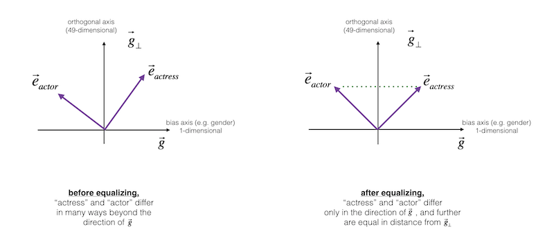
Equalize pairs

In the final equalization step, what we’d like to do is to make sure that words like grandmother and grandfather are both exactly the same similarity, or exactly the same distance, from words that should be gender neutral, such as babysitter or such as doctor.
The key idea behind equalization is to make sure that a particular pair of words are equi-distant from the 49-dimensional g⊥.

修心问道

Deep Learning-3-2 Natual Language Processing & Word Embeddings