Deep Learning-3-1 Recurrent Neural Networks

Learning Objectives

• Why sequence models
• Notation
• Recurrent neural network model
• Language model and sequence generation
• Vanishing gradients with RNNs
• Gated Recurrent Unit (GRU)
• Long Short Term Momory (LSTM)
• Bidirectional RNN
• Deep RNNs

---

Why sequence models

Examples of sequence data:

• Speech recognition
• Music generation
• Sentiment classification
• DNA sequence analysis
• Machine translation
• Video activity recognition
• Named entity recognition

Notation

For a motivation, in the problem of Named Entity Recognition (NER), we have the following notation:

• $x$ is the input sentence, such as: Harry Potter and Hermione Granger invented a new spell.
• $y$ is the output, in this case: 1 1 0 1 1 0 0 0 0.
• $x^{<t>}$ denote the word in the index t and $y^{<t>}$ is the correspondent output.
• In the i-th input example, $x^{(i)<t>}$ is t-th word and $T^{x(i)}$ is the length of the i-th example.
• $T_y$ is the length of the output. In NER, we have $T_x = T_y$.

Words representation introduced in this video is the One-Hot representation.

• First, you have a dictionary which words appear in a certain order.
• Second, for a particular word, we create a new vector with 1 in position of the word in the dictionary and 0 everywhere else.

For a word not in your vocabulary, we need create a new token or a new fake word called unknown word denoted by <UNK>.

Recurrent Neural Network Model

If we build a neural network to learn the mapping from $x$ to $y$ using the one-hot representation for each word as input, it might not work well. There are two main problems:

1. Inputs and outputs can be different lengths in different examples. not every example has the same input length $T_x$ or the same output length $T_y$. Even with a maximum length, zero-padding every input up to the maximum length doesn’t seem like a good representation.
2. For a naive neural network architecture, it doesn’t share features learned across different positions of texts.

Recurrent Neural Networks:

• A recurrent neural network does not have either of these disadvantages.
• At each time step, the recurrent neural network that passes on as activation to the next time step for it to use.
• The recurrent neural network scans through the data from left to right. The parameters it uses for each time step are shared.
• One limitation of unidirectional neural network architecture is that the prediction at a certain time uses inputs or uses information from the inputs earlier in the sequence but not information later in the sequence.
  • He said, "Teddy Roosevelt was a great president."
  • He said, "Teddy bears are on sale!"
  • You can’t tell the difference if you look only at the first three words.!

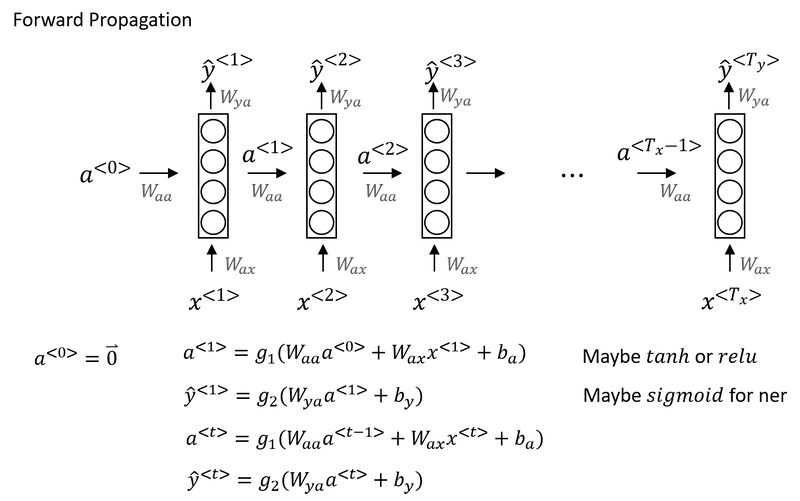
Instead of carrying around two parameter matrices $W_{aa}$ and $W_{ax}$, we can simplifying the notation by compressing them into just one parameter matrix $W_a$.

Backpropagation through time

In the backpropagation procedure the most significant messaage or the most significant recursive calculation is which goes from right to left, that is, backpropagation through time.

Different types of RNNs

There are different types of RNN:

• One to One
• One to Many
• Many to One
• Many to Many

Language model and sequence generation

So what a language model does is to tell you what is the probability of a particular sentence.

For example, we have two sentences from speech recognition application:

Sentence	Probability
The apple and pair salad.	𝑃(The apple and pair salad)=$3.2 \times 10^{-13}$
The apple and pear salad.	𝑃(The apple and pear salad)=$5.7\times 10^{-10}$

For language model it will be useful to represent a sentence as output y rather than inputs x. So what the language model does is to estimate the probability of a particular sequence of words $𝑃(y<1>, y<2>, …, y<T_y>)$.

How to build a language model?

Cats average 15 hours of sleep a day <EOS> Totally 9 words in this sentence.

• The first thing you would do is to tokenize this sentence.
• Map each of these words to one-hot vectors or indices in vocabulary.
  • Maybe need to add extra token for end of sentence as <EOS> or unknown words as <UNK>.
  • Omit the period. if you want to treat the period or other punctuation as explicit token, then you can add the period to you vocabulary as well.
• Set the inputs $x^{<t>}$ = $y^{<t-1>}$`.
• What a<1> does is it will make a softmax prediction to try to figure out what is the probability of the first words y<1>. That is what is the probability of any word in the dictionary. Such as, what’s the chance that the first word is Aaron?
• Until the end, it will predict the chance of <EOS>.
• Define the cost function. The overall loss is just the sum over all time steps of the loss associated with the individual predictions.

If you train this RNN on a large training set, we can do:

• Given an initial set of words, use the model to predict the chance of the next word.
• Given a new sentence y<1>,y<2>,y<3>, use it to figure out the chance of this sentence: p(y<1>,y<2>,y<3>) = p(y<1>) * p(y<2>|y<1>) * p(y<3>|y<1>,y<2>)

Sampling novel sequences

After you train a sequence model, one way you can informally get a sense of what is learned is to have it sample novel sequences.

How to generate a randomly chosen sentence from your RNN language model:

• In the first time step, sample what is the first word you want your model to generate: randomly sample according to the softmax distribution.
  • What the softmax distribution gives you is it tells the chance of the first word is ‘a’, the chance of the first word is ‘Aaron’, the chance of the first word is ‘Zulu’, or the chance of the first word refers to <UNK> or <EOS>. All these probabilities can form a vector.
  • Take the vector and use np.random.choice to sample according to distribution defined by this vector probabilities. That lets you sample the first word.
• In the second time step, remember in the last section, y<1> is expected as input. Here take ŷ<1> you just sampled and pass it as input to the second step. Then use np.random.choice to sample ŷ<2>. Repeat this process until you generate an <EOS> token.
• If you want to make sure that your algorithm never generate <UNK>, just reject any sample that come out as <UNK> and keep resampling from vocabulary until you get a word that’s not <UNK>.

Character level language model:

If you build a character level language model rather than a word level language model, then your sequence y1, y2, y3, would be the individual characters in your training data, rather than the individual words in your training data. Using a character level language model has some pros and cons. As computers gets faster there are more and more applications where people are, at least in some special cases, starting to look at more character level models.

Advantages:

• You don’t have to worry about <UNK>.

Disadvantages:

• The main disadvantage of the character level language model is that you end up with much longer sequences.
• And so character language models are not as good as word level language models at capturing long range dependencies between how the the earlier parts of the sentence also affect the later part of the sentence.
• More computationally expensive to train.

Vanishing gradients with RNNs

• One of the problems with a basic RNN algorithm is that it runs into vanishing gradient problems.
• Language can have very long-term dependencies, for example:
  • The cat, which already ate a bunch of food that was delicious …, was full.
  • The cats, which already ate a bunch of food that was delicious, and apples, and pears, …, were full.
• The basic RNN we’ve seen so far is not very good at capturing very long-term dependencies. It’s difficult for the output to be strongly influenced by an input that was very early in the sequence.
• When doing backprop, the gradients should not just decrease exponentially, they may also increase exponentially with the number of layers going through.
• Exploding gradients are easier to spot because the parameters just blow up and you might often see NaNs, or not a numbers, meaning results of a numerical overflow in your neural network computation.
  • One solution to that is apply gradient clipping: it is bigger than some threshold, re-scale some of your gradient vector so that is not too big.
• Vanishing gradients is much harder to solve and it will be the subject of GRU or LSTM.

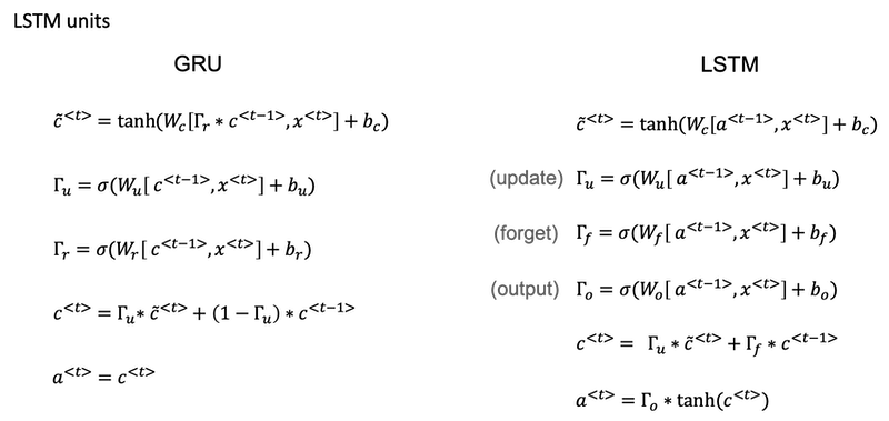
Gated Recurrent Unit (GRU)

Gate Recurrent Unit is one of the ideas that has enabled RNN to become much better at capturing very long range dependencies and has made RNN much more effective.

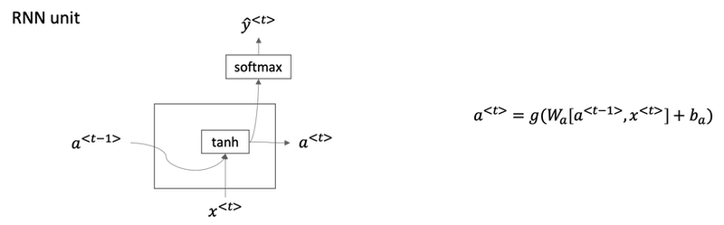
A visualization of the RNN unit of the hidden layer of the RNN in terms of a picture:

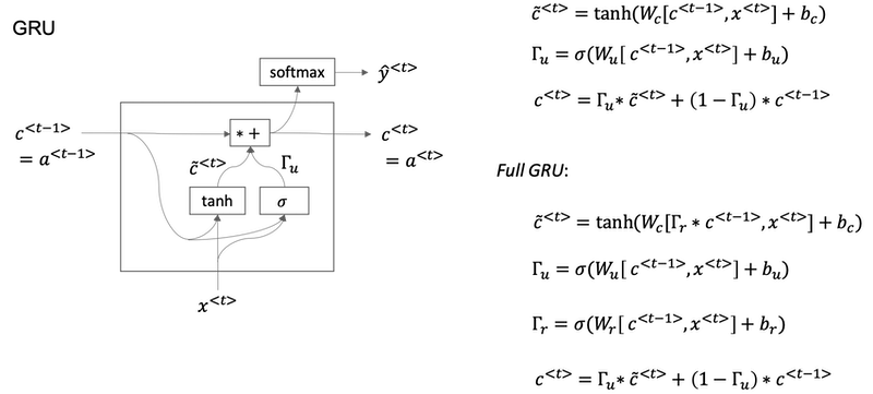
• The GRU unit is going to have a new variable called c, which stands for memory cell.
• c̃<t> is a candidate for replacing c<t>.
• Since a sigmoid function is applied to calculate Γu, at most of the time Γu is either close to 0 or 1. For intuition, think of Γu as being either zero or one most of the time. In practice gamma won’t be exactly zero or one.
• Because Γu can be so close to zero, can be 0.000001 or even smaller than that, it doesn’t suffer from much of a vanishing gradient problem
• Because when Γu is so close to zero this becomes essentially c<t> = c<t-1> and the value of c is maintained pretty much exactly even across many many time-steps. So this can help significantly with the vanishing gradient problem and therefore allow a neural network to go on even very long range dependencies.
• In the full version of GRU, there is another gate Γr. You can think of r as standing for relevance. So this gate Γr tells you how relevant is c<t-1> to computing the next candidate for c<t>.

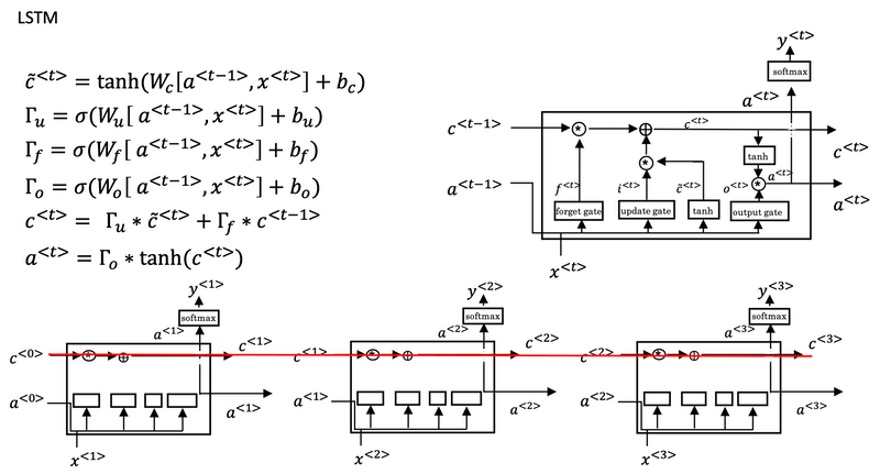
Long Short Term Memory (LSTM)

• For the LSTM we will no longer have the case that a<t> is equal to c<t>.
• And we’re not using relevance gate Γr. Instead, LSTM has update, forget and output gates, Γu, Γf and Γo respectively.

One cool thing about this you’ll notice is that this red line at the top that shows how, so long as you set the forget and the update gate appropriately, it is relatively easy for the LSTM to have some value c<0> and have that be passed all the way to the right to have your, maybe, c<3> equals c<0>. And this is why the LSTM, as well as the GRU, is very good at memorizing certain values even for a long time, for certain real values stored in the memory cell even for many, many timesteps.

One common variation of LSTM:

• Peephole connection: instead of just having the gate values be dependent only on a<t-1>, x<t>, sometimes, people also sneak in there the values c<t-1> as well.

GRU vs. LSTM:

• The advantage of the GRU is that it’s a simpler model and so it is actually easier to build a much bigger network, it only has two gates, so computationally, it runs a bit faster. So, it scales the building somewhat bigger models.
• The LSTM is more powerful and more effective since it has three gates instead of two. If you want to pick one to use, LSTM has been the historically more proven choice. Most people today will still use the LSTM as the default first thing to try.

Implementation tips:

• forget gate Γf

  • The forget gate Γf<t> has the same dimensions as the previous cell state c<t-1>.
  • This means that the two can be multiplied together, element-wise.
  • Multiplying the tensors Γf<t> is like applying a mask over the previous cell state.
  • If a single value in Γf<t> is 0 or close to 0, then the product is close to 0.
    • This keeps the information stored in the corresponding unit in c<t-1> from being remembered for the next time step.
  • Similarly, if one value is close to 1, the product is close to the original value in the previous cell state.
    • The LSTM will keep the information from the corresponding unit of c<t-1>, to be used in the next time step.

• candidate value c̃<t>

  • The candidate value is a tensor containing information from the current time step that may be stored in the current cell state c<t>.
  • Which parts of the candidate value get passed on depends on the update gate.
  • The candidate value is a tensor containing values that range from -1 to 1. (tanh function)
  • The tilde “~” is used to differentiate the candidate c̃<t> from the cell state c<t>.

• update gate Γu

• The update gate decides what parts of a “candidate” tensor c̃<t> are passed onto the cell state c<t>.

• The update gate is a tensor containing values between 0 and 1.

  • When a unit in the update gate is close to 1, it allows the value of the candidate c̃<t> to be passed onto the hidden state c<t>.
  • When a unit in the update gate is close to 0, it prevents the corresponding value in the candidate from being passed onto the hidden state.

• cell state c<t>

  • The cell state is the “memory” that gets passed onto future time steps.
  • The new cell state c<t> is a combination of the previous cell state and the candidate value.

• output gate Γo

  • The output gate decides what gets sent as the prediction (output) of the time step.
  • The output gate is like the other gates. It contains values that range from 0 to 1.

• hidden state a<t>

  • The hidden state gets passed to the LSTM cell’s next time step.
  • It is used to determine the three gates (Γf, Γu, Γo) of the next time step.
  • The hidden state is also used for the prediction y<t>.

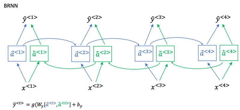
Bidirectional RNN

• Bidirectional RNN lets you at a point in time to take information from both earlier and later in the sequence.
• This network defines a Acyclic graph
• The forward prop has part of the computation going from left to right and part of computation going from right to left in this diagram.
• So information from x<1>, x<2>, x<3> are all taken into account with information from x<4> can flow through a backward four to a backward three to Y three. So this allows the prediction at time three to take as input both information from the past, as well as information from the present which goes into both the forward and the backward things at this step, as well as information from the future.
• Blocks can be not just the standard RNN block but they can also be GRU blocks or LSTM blocks. In fact, BRNN with LSTM units is commonly used in NLP problems.

Disadvantage:
The disadvantage of the bidirectional RNN is that you do need the entire sequence of data before you can make predictions anywhere.

So, for example, if you’re building a speech recognition system, then the BRNN will let you take into account the entire speech utterance but if you use this straightforward implementation, you need to wait for the person to stop talking to get the entire utterance before you can actually process it and make a speech recognition prediction. For a real type speech recognition applications, they’re somewhat more complex modules as well rather than just using the standard bidirectional RNN as you’ve seen here.

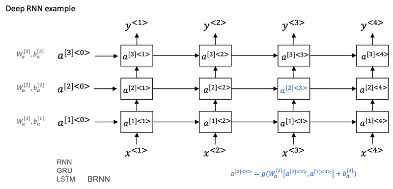
Deep RNNs

• For learning very complex functions sometimes is useful to stack multiple layers of RNNs together to build even deeper versions of these models.
• The blocks don’t just have to be standard RNN, the simple RNN model. They can also be GRU blocks LSTM blocks.
• And you can also build deep versions of the bidirectional RNN.