Learning Objectives
- Visualization of Neural Networks
- Gradient-Based Visualizations
- Optimizing the Input Images
- Testing Robustness
- Style Transfer
Visualization of Neural Networks
Given a model we would like to understand what it has learned. Given some random initialization values what values has it arrived at, or converged, or trained, to? After optimization it should have found set of optimal values. For Linear classifiers we can take the learned weights, reshape them into images, and then plot them in a normalized way. This gives us a picture of the weight template used to classify objects.
For convoutional layers the kernels are the weights. Recall that the kernel is convolved with the image in a repeated process of step size = stride. So high response values from the covolution are indicative of similarity.
We can also plot the activations after running a kernel across an image. Each activation layer yields an output map (aka feature map, activation map). These maps represent spatial location with high values that highly correlate with the kernel. think of an edge map for example.
Using Gradients and gradient stats let us understand wht the model is learning.
Finally we can look at the robustness of the Network to determine any weak points.
For FC layers, if the nodes are connected to the image itself, then you can simply reshape the weights, normalize(0-255) and view as an image.
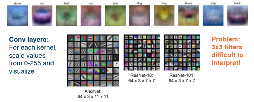
What’s interesting about these are that they began life as purely random values, ie at initialization they would look like a speckled image for example. By now they begin to resemble patterns, or templates, with colour and textures. of course the smaller the kernel the smaller the image so they can be difficult at times.
Visualizing activation/filter maps can be a lot trickier.
:warning: Problem: Small convolution outputs are hard to visualize/interpret.
We can take the activations of any layer (FC, conv, etc) and perfrom dimensionality reduction.
- This can be used to reduced to two dimensions for ploting.
- One option is to use Principle Component Analysis (PCA).
- PCA is a dimensionality reduction method that is often used to reduce the dimensionality of large data sets, by transforming a large set of variables into a smaller one that still contains most of the information in the large set.
- The other option is tSNE, which performs a nonlinear mapping while preserving pair-wise distances.
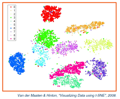
The better that these groups are seperated the better the classifier will perform.
Summary and Caveats
While these methods provide some visual interpretation this is highly biased on the interpreter and can often be misleading, or simply uninformative.
- Assessing interpretability is difficult
- It requires user studies to show usefulness
- E.g. they allow a user to predict mistakes beforehand
- Neural Networks learn distributed representation
- That means they don’t learn a feature/point. The nodes don’t really represent any feature either. A node that is activated for a face may also be activated for bird (silly example), the point being that a node that is good for one trait may also effect other traits.
- This adds to the difficulty of interpretation.
In a nutshell: Visualizations help provide some guidance and direction. They are not conclusive on their own.
Gradient-Based Visualizations
Gradient of Loss w.r.t. Image
Recall that the backwards pass gives us the gradients for all layers: How the loss changes as we change the different parts of the input. This is useful not only for optimization but also to understand what was learned.
- Gradient of the loss w.r.t all layers ( including the input!).
- Gradient of any layer w.r.t. input (by cutting off the computation graph)
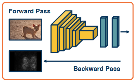
Here is the idea:
- It helps us to understand the sensitivity of the loss to the input
- Large sensitivity implies a high pixel importance (Saliency Maps)
In practice:
- Instead of the loss, we find the gradient of classifier scores (pre softmax).
- It should be noted that the softmax introduces some complexity which can affect the loss gradients, hence why we take the scores before the softmax.
- Take the absolute value of the gradient.
- Sum across all the channels (channels don’t matter).
Object Segmentation
Applying traditional computer vision (CV) methods and algorithms on the gradients can get us object segmentation for free.
Surprising because this is not really part of the supervision process.
This can be used to detect dataset bias. For example the presence of snow might be used by a model to detect the presence of a wolf. And so even a missclassification or incorrect prediction can be informative. Looking at the gradients and using them to create a segmentation would yield the presence of snow, indicating the bias.
Gradient of Activation w.r.t. Input
Rather than loss or score, we can pick a neuron somewhere deep in the network and compute the gradient of the activation w.r.t. the input.
Setps:
- Pick a neuron – somewhere in the network say 3rd conv layer
- Find the gradient of its activation wrt the input image – run the forward pass up until that point/layer
- Can first find the highest activated image patches using it’s corresponding neuron (based on the receptive field)
:warning: It should be stressed that the way we’ve been using backprop up until now may not be good for visualizing.
For example, when visualizing we may get parts of an image that decrease the feature activation. So you can get parts of an image with negative gradients. You want to focus on areas with a positive influence/gradients
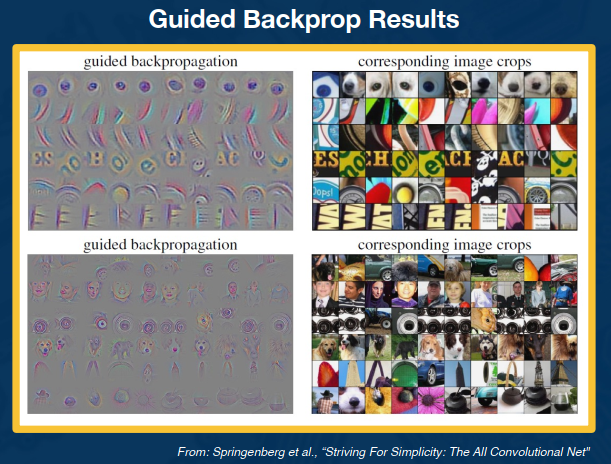
Guided backprop
Guided backprop can be used to improve visualizations.
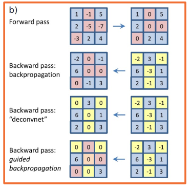
In the above figure:
- Forward pass: positive values remain, negatives get zero’d out
- Backwards pass: “deconvnet” (composed of deconvolution and unpooling layers), only positve values are passed back and negative influence are removed
- Backwards pass: Guided backprop, this is both the forward pass and the deconvnet applied, and only positive influences remain and get propogated
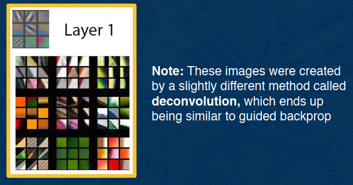
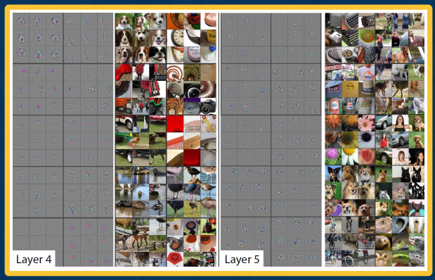
VGG Layer-by-Layer Visualization
VGG is another method also which can produce similar results.
VGG stands for Visual Geometry Group; it is a standard deep Convolutional Neural Network (CNN) architecture with multiple layers. The “deep” refers to the number of layers with VGG-16 or VGG-19 consisting of 16 and 19 convolutional layers.
In the first layer of a neural network, it produces what could best be described as edge orientation outputs. It may also learn things like color or textual patterns. In general, however, it tends to find low level features.
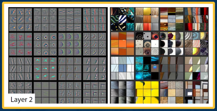
In the second layer we’ll see that these low level features such as edges are combined in order to find higher level features such as motifs, (Corners, circles, shapes, etc), as well as more interesting patterns and textures.
In layer 3 we get more abstract. We find things like wheels of a car or different parts of people.
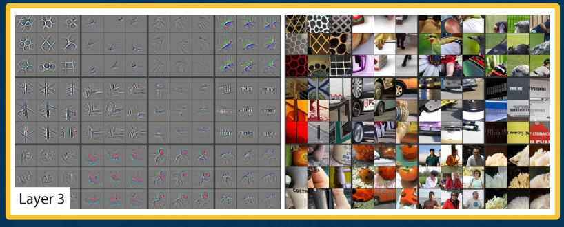
By layer 4 and 5 we are nearing our templates. Here we may have the entire object being detected, or at the very least more than just one part as may have been located using layer 3.
Guided Grad-CAM
As researchers began plotting more and more saliency maps, more and more sophisticated methods began to emerge to understand what neural networks consider to be important. One of these methods is the Grad-CAM.
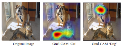
GradCAM trys to determine where a CNN is looking at in order to come to a decision. It can be used for
- Weakly supervised localization: Determining the location of an object using a model trained on whole image labels rather than explicit location annotations
- Weakly supervised segmentation: Where the model predicts all the pixels that belong to an particular object without requiring pixel level labels for training.
GradCAM is a form of post-hoc attention. Meaning that it is a method for producing heatmaps that are applied to an already trained (pretrained/prebuilt) neural network after training is complete and the parameters are fixed. (Whereas trainable attention refers to the production of a heat map in the building/training phase.
Summary
- Gradients are important not just for optimization, but also for analyzing what neural networks have learned
- Standard backprop not always the most informative for visualization purposes
- Several ways to modify the gradient flow to improve the visualization results
Optimizing the Input Images
Idea: Since we have the gradient of scores w.r.t. inputs, can we optimize the image itself to maximize the score?
Why?
- Create images from scratch
- Adversarial examples (maliciously crafted inputs that are specifically designed to deceive machine learning models)
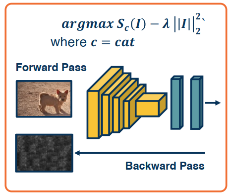
We do this by performing gradient ascent on an image.
- Start from a random, or zero, image
- Compute the forward pass and gradients
- Perform ascent
- Iterate (repeat 2 previous steps)
- Be sure to use scores to avoid minimizing other class scores (after we compute the softmax probabilities)
- Because we’re using the raw scores themselves, the network is forced to directly increase the score for the class that we care about.
- We will often need some form of regularization term to induce statistics of natural imagery
- e.g. small pixel values or spatial smoothness
Consider the following image. While less than optimal you can see that there is the formulation of an image.
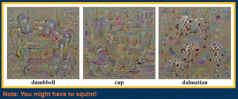
We can improve these results with various tricks:
- Clipping of small values and gradients
- Gaussian blurring
- Other techiques exist as well
Summary
We can optimize the input image to generate examples to increase class
scores or activations.
This can show us a great deal about what examples (not in the training set) activate the network.
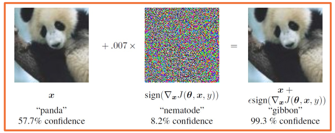
Testing Robustness
- We can perform gradient ascent on image
- Rather than start from zero image, why not real image?
- And why not optimize the score of an arbitrary (incorrect!) class
It turns out that only a very small number of pixels (per dimension) is needed to optimize the incorrectness. By adding a bit of noise or perturbations we can cause a network to misclassify.
This problem is not unique to Deep Learning/Machine Learning!
- Other classical methods can suffer from it as well
- Can show how linearity (even at the end) can bring this about
- can add many small values that add up in the right direction
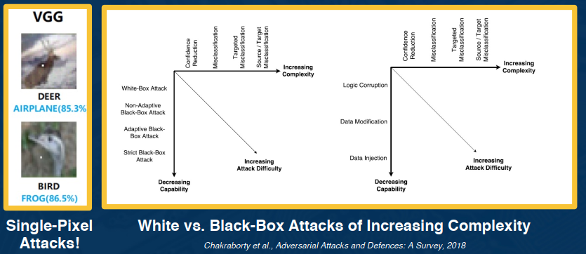
Summary of Adversarial Attacks & Defenses
Similar to other security related areas, it’s very much a cat and mouse game.
Some defenses exist and their performance/success depends on the situation, such as:
- Training with adversarial examples
- Perturbations, noise, or re-encoding of inputs
There are no universal methods however that exist, are robust, to all types of attacks.
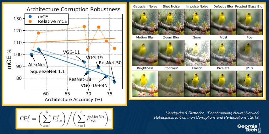
Other forms of Robustness Testing
We can try to understanding the biases of CNNs (compare to those of humans)
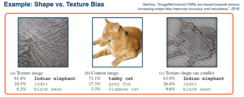
In the example, a human can discern that a cat with the texture of an elephant is still a cat, but a NN will almost certainly classify it as an elephant.
Summary
- Various ways to test the robustness and biases of neural networks
- Adversarial examples have implications for understanding and trusting them
- Exploring the gain of different architectures in terms of robustness and biases can also be used to understand what has been learned.
Style Transfer
This refers to the generation of an image where the content of the target image remains the same but the style, or texture, is transfered from another image.
Images can be generated through backpropogation – Regularization can be used to ensure we match image statisitcs.
Idea: What if we want to preserve the content of a particular image?
- We can match the features at different layers
- We can even construct a loss for this
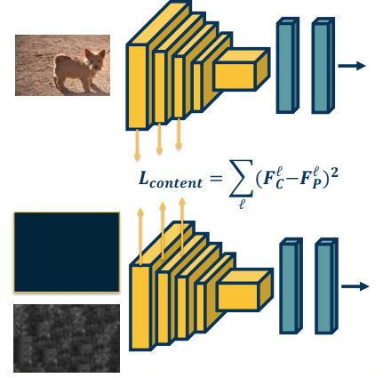
Example: Suppose we have an image of a dog that we wish to replicate
- We feed the image through a CNN
- In doing so, we extract the activation layers and feature values for all the layers
- We then compute the loss
- The loss can be defined as the difference between the features of generate layer and the content image
- $L_{content}=(F_C^1-F_P^1)^2$
- What’s happening here is that we are minimizing the loss in the feature space
- You could use something other than features but the principle would remain the same
We can take this another step forward as well! Recall that backwards edges are going to the same node are summed. So we can take the loss at each of the layers and sum them up:
$$
L_{content}=\sum_l (F_C^l-F_P^l)^2
$$
Idea: Can we have the content of one image and texture (style) of another image?
Yes! The idea here is very similar to the process above. We start with 2 images, let’s call them the content and the style image. We compute the feature maps or activations. We also create a third image from scratch, from nothing. Now want we need to do is to minimize the loss between our zero image and each of the feature layers of the style and content images. It should be clear these need to be minimized together, at the same time. But we can’t use the same loss on both sides. Otherwise you’ll get converging content or converging styles, not a mix of both which is what we want.
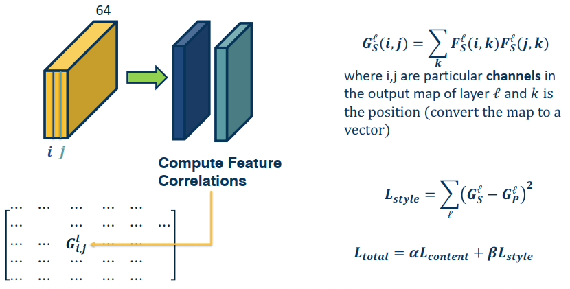
How do we represent similarity in terms of textures?
- There is a history of this in classical Computer vision.
- Key ideas revolve around summary statisitcs
- Should ideally remove most spatial information
- Deep Learning variants
- Called a Gram Matrix
Summary
- Generating images through optimization is a powerful concept!
- Besides fun and art, methods such as stylization also useful for understanding what the network has learned
- Also useful for other things such as data augmentation

