Learning Objectives
- Backwards Pass
- Convolution Gradients
- Simple Convolutional Neural Networks
- Advanced Convolutional Networks
- Transfer Learning & Generalization
Backwards Pass for Convolution Layer
It is instructive to calculate the backwards pass of a convolution layer. Similar to fully connected layer, it will be simple vectorized linear algebra operation! We will see a duality between cross-correlation and convolution.
Let’s recap the cross-correlation. It is defined as:
$$
S(r,c) = (I * K)(r,c) = \sum_{a=0}^{k_1-1} \sum_{b=0}^{k_2-1} I(r+a,c+b)K(a,b)
$$
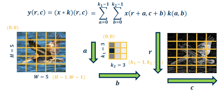
So $|y|=H \times W$
What is $\frac{\partial L}{\partial y}$? Assume size $H \ times W$ (add padding for convenience)
$$\frac{\partial L}{\partial y(r,c)}$$ to access the element
Similar to before we can now compute the gradients using our friend the chain rule
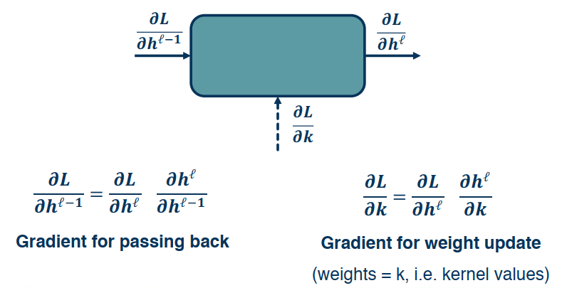
Important Note: The right side gradients are for the weight update, which in this case is the kernel values.
Gradient for Convolution Layer
Gradient for weight update
Let’s look at the gradient for weight update.
We could calculate one pixel at a time using $\frac{\partial L}{\partial k(a,b)}$. It may not be explicit here but this will effect every pixel in the output, because the kernel is being strided across the image. This means that the gradient flow will be affecting every output pixel. Meaning we need to incorporate all the upstream gradients.
For all upstream gradients, we have:
$$
{\frac{\partial L}{\partial y(0,0)}, \frac{\partial L}{\partial y(0,1)}, …,\frac{\partial L}{\partial y(H,W)}}
$$
Apply the chain rule to sum over all output pixels, yields:
$$
\frac{\partial L}{\partial k(a’,b’)} = \sum_{r=0}^{H-1}\sum_{c=0}^{W-1} \frac{\partial L}{\partial y(r,c)} \frac{\partial y(r,c)}{\partial k(a’, b’)}
$$
Now we observe that
$$
\frac{\partial y(r,c)}{\partial k(a’, b’)} = x(r+a’, c+b’)
$$
Therefor, we have
$$
\frac{\partial L}{\partial k(a’,b’)} = \sum_{r=0}^{H-1}\sum_{c=0}^{W-1} \frac{\partial L}{\partial y(r,c)} x(r+a’, c+b’)
$$
Looking at this we can see that it is the cross correlation between the upstream gradient and the input.
Gradient for passing back
Let’s derive the loss analytically. Chain rule for affected pixels (sum gradients):
$$
\frac{\partial L}{\partial x(r’,c’)}=\sum_{Pixels\ p} \frac{\partial L}{\partial y(p)} \frac{\partial y(p)}{\partial x(r’, c’)}
$$
$$
\frac{\partial L}{\partial x(r’,c’)}=\sum_{a=0}^{k_1-1} \sum_{b=0}^{k_2-1} \frac{\partial L}{\partial y(r’-a, c’-b)} \frac{\partial y(r’-a, c’-b)}{\partial x(r’,c’)}
$$
Using the definition of cross-correlation (use a’, b’ to distinguish from prior variables).
$$
y(r’,c’) = (x * k)(r’,c’) = \sum_{a’=0}^{k_1-1} \sum_{b’=0}^{k_2-1} x(r’+a’,c’+b’)k(a’,b’)
$$
Plug in what we actually wanted:
$$
y(r’-a,c’-b) = (x * k)(r’,c’) = \sum_{a’=0}^{k_1-1} \sum_{b’=0}^{k_2-1} x(r’-a+a’,c’-b+b’)k(a’,b’)
$$
What is $\frac{\partial y(r’-a, c’-b)}{\partial x(r’,c’)}$? Well, it turns out this is just $k(a,b)$. (We want term with $x(r’, c’)$ in it, this happens when a’=a and b’=b.)
Plugging in to earilier equation:
$$
\frac{\partial L}{\partial x(r’,c’)}=\sum_{a=0}^{k_1-1} \sum_{b=0}^{k_2-1} \frac{\partial L}{\partial y(r’-a, c’-b)} \frac{\partial y(r’-a, c’-b)}{\partial x(r’,c’)} = \sum_{a=0}^{k_1-1} \sum_{b=0}^{k_2-1} \frac{\partial L}{\partial y(r’-a, c’-b)} k(a,b)
$$
Hopefully this looks familiar? It’s the convolution between the upstream gradient and the kernel. Which we can implement by just flipping the kernel and applying cross correlation. And again, all operations can be implemented via matrix multiplications, just as we do in a fully connected layer.
Simple Convolutional Neural Networks
Since the output of a convolution and a pooling layers are (multi-channel) images, we can sequence them just as any other layer.
For example: Image –> Convolution (+NonLinear Layer) –> Pooling –> ??
In the last position we can perform a (convolution –> pooling) a second time or create a fully connected layer.
Here’s a depiction of a simple CNN. The end goal is to have a more useful but lower dimensional set of features to feed into our fully connected layer. Which should simply result in some classifier.
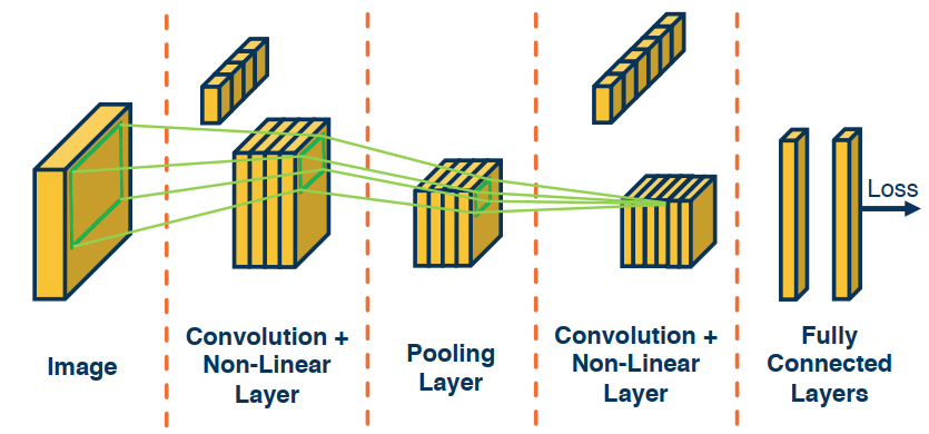
Now we have an end to end CNN, that starts with a raw input, the extracts more and more abstract/meaningful features, that finally are fed into an FC to obtain a prediction. Through the loss we will be able to trace back our gradient flow, update weights/kernel and push them backwards until we get to the raw image.
Effectively we are optimizing our kernels to minimize the loss at all stages.
One side effect that should be noted is the increasing reseptive field for a pixel as you move backwards in the process. This should not come as a surprise as pooling, and convolution, can reduce the input.
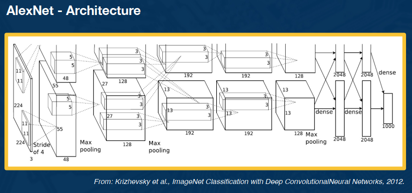
Advanced Convolutional Networks
Here is the cutting edge CNN architecture ( Back in 2012 ):
Key aspects were:
- ReLU instead of sigmoid or tanh
- Specialized normalization layers
- PCA-based data augmentation
- Dropout
- Ensembling
Other aspects include:
- 3x3 convolution (stride of 1, padding of 1)
- 2x2 max pooling (stride 2)
- High number of parameters
These can be pretty memory intensive though.
Transfer Learning & Generalization
Generalization
How can we generalize our learning (from training to testing dataset). We will also discuss transfer learning which can significantly reduce the amount of labelled data that we need to fit the large number of parameters that we will have in these very complex networks.
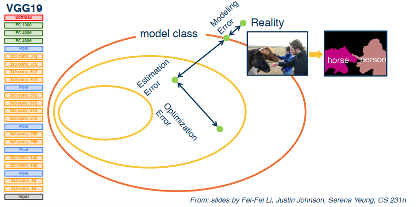
In any model construction process there will be several sources of error that prevent you from fully modelling the real world.
- Optimization error
- Estimation error
Transfer Learning
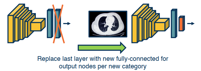
What if we don’t have a lot, or enough, data? We can reuse our data.
- Step 1: Train on a large scale data set (like imagenet)
- Step 2: Take your custom data and initialize the network with weights trained in step 1
- Step 3: Continue to train on new data
- Finetune: Update all parameters
- Freeze feature layer: Update only the last layer weights (used when there’s not enough data)
This works surprisingly well! Features learned for 1000 object categories will work well for the 1001st! It also generalizes across tasks, ie from classification to object detection.
Learning with less labels, doesn’t work out well though.
- If the source dataset you train on is very different from the target dataset, transfer learning is not as effective
- If you have enough data for the target domain it will simply result in faster convergence.

