Learning Objectives
- Convolutional Neural Networks
- Convolution Layers
- Input & Output Sizes
- Pooling Layers
Convolutional Neural Networks
Until now we’ve focused exclusively on linear and nonlinear layers. We’ve also discussed at length fully connected layers (FCs) where all output layers are connected to all input nodes. Of course, these are not the only types of layers and in this section we will begin exploring another type: Convolutional Neural Networks.
Layers don’t need to be fully connected!! For example, when building image based models it tends to make more sense to look at areas of an image rather than look at each pixel individually. So we might define nodes to focus on small patches of inputs, or windows. To approach this we consider the idea of convolution operations as a layer in the neural network.
Recall the idea of convolution. A convolution is a process whereby a Kernel(matrix) is multiplied against a matrix(window), this process is repeated for ALL possible windows in the target dataset (usually an image). The reason this is so beneficial is that kernal can be created to extract features from an image.
Properties of Convolutions
Sparse Interactions: (aka Sparse Weights, Sparse connectivity) This happens when the kernel K is smaller than the input. If there are M inputs and N outputs, then matrix multiplication requires MxN parameters and thus the complexity is O(MxN). If we limit the output to KxN where K < M then we can reduce the complexity by the same amount to O(KxN)
Parameter Sharing: This refers to the use of the same parameter for more than one function in a model.
Equivariance: To say a function is equivariant means that if the input changes, then the output changes in the same way. i.e. f(g(t))=g(f(t))
Convolution Operations
Here are some examples of convolutions.
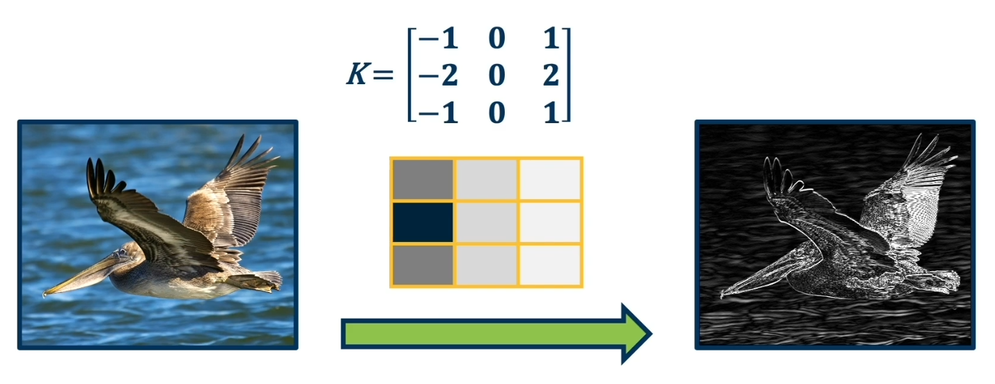
This new convolution layer can take any input 3D tensor (say, RGB) and output another similarly shaped output. In fact what we will be looking to do is to use/apply multiple kernels for various features we want to extract. We will also need to take the output of these convolutions and organize them into feature maps so our neural network may perform the needed analysis.
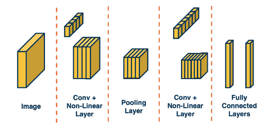
Convolution layers can be combined with non-linear and pooling layers which reduce the dimensionality of the data. For example we can take a 3x3 patch from an image and take the max. This effectively reduces 9 numbers down to 1.
The following image gives a high level approach to convolutional neural networks. The idea is to extract more and more abstract features from the image/data. Finally in the end we create our fully connected layer (one or multiple) to produce our results. Hopefully by the time we get to the last stage our tensors have been reduces to a manageable size.
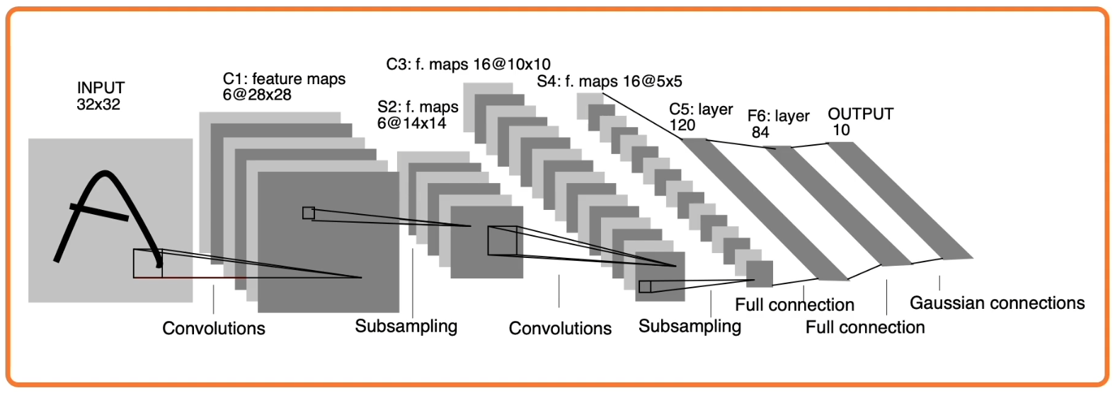
Here is a more advanced example of the type of architecture that is used in practice. These have existed since the 1980’s. One application of these has been to read scanned checks cashed in a bank. (Note that a Gaussian Connection is just a fully connected layer)
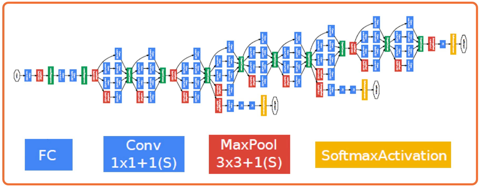
Nowadays these have become much more complex.
Convolution Layers
Backpropagation, and automatic differentiation, allows us to optimize any function composed of differentiable blocks.
- No need to modify the learning algorithm
- The complexity of the function is limited only by computation and memory
However, connectivity in linear layers doesn’t always make sense! Consider for example a 1024x1024 image, assuming it’s greyscale then that’s 1,048,576 pixels and therefore we need 1million by N weights plus another N bias terms just so we can properly feed it into a fully connected layer. This begs the question: Is this really necassary?
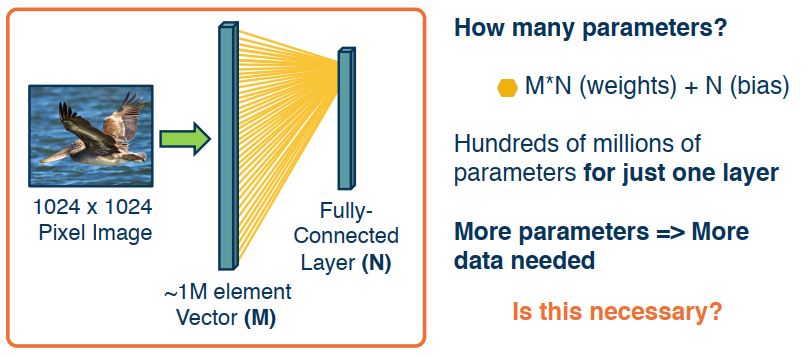
Image features are spatially localized!
- Image features tend to be smaller features repeated across the image.
- For example Edges, Colors, motifs (corners).
- No reason to believe one feature tends to appear in one location vs. another (stationarity).
How can we induce a bias in the design of a neural network layer to reflect this?
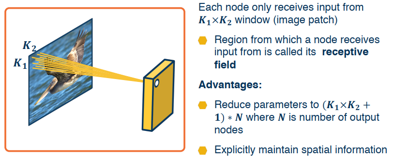
Idea 1: Receptive fields
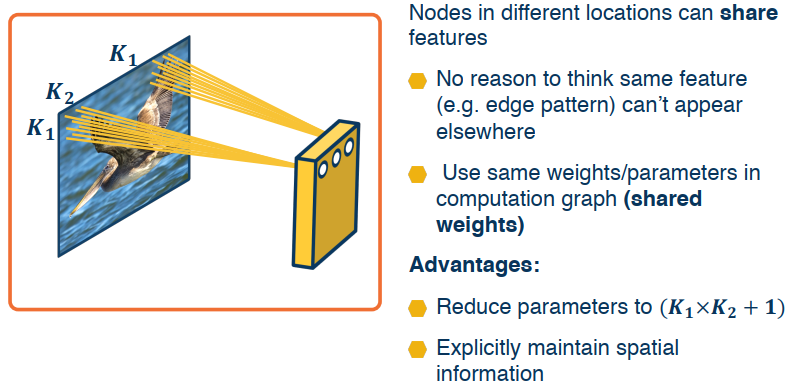
Idea 2: Shared Weights
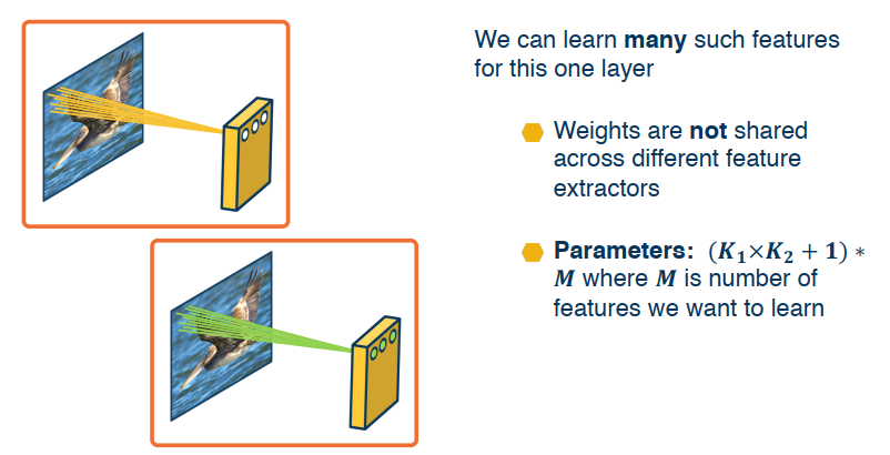
Idea 3: Learning Many Features
Convolution Review
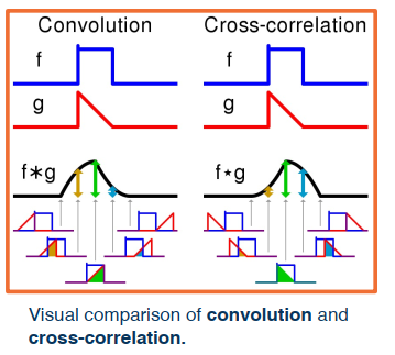
In mathematics a convolution is an operation on two functions f and g producing a third function that is typically viewed as a modified version of one of the original functions, giving the area of overlap between the two functions as a function of the amount that one of the original functions is translated.
In terms of deep learning, an (image) convolution is an element-wise multiplication of two matrices followed by a sum.
Seriously. That’s it. You just learned what a convolution is:
- Take two matrices (which both have the same dimensions).
- Multiply them, element-by-element (i.e., not the dot product, just a simple multiplication).
- Sum the elements together.
There is also a highly similar and important related operation called cross correlation.
Convolutions versus cross correlation
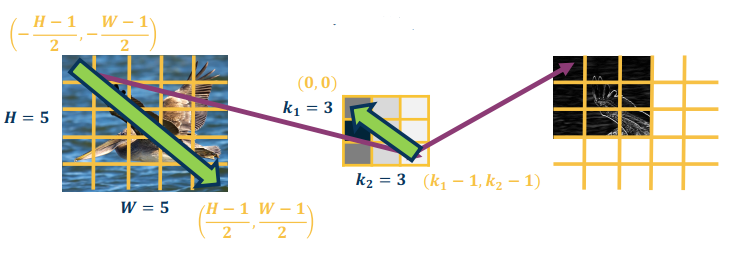
Convolution (denoted by the * operator) over a two-dimensional input image I and two-dimensional kernel K is defined as:
$$
S(r,c) = (I * K)(r,c) = \sum_{a=-\frac {k_1-1}{2}}^{\frac {k_1-1}{2}} \sum_{-\frac {k_2-1}{2}}^{\frac {k_2-1}{2}} I(r-a,c-b)K(a,b)
$$
However, many machine learning and deep learning libraries use the simplified cross-correlation function
$$
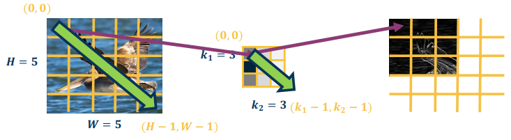
S(r,c) = (I * K)(r,c) = \sum_{a=0}^{k_1-1} \sum_{b=0}^{k_2-1} I(r+a,c+b)K(a,b)
$$
where $k_1, k_2$ are the row and column number of the kernal, and $I, K$ are the input matrix and kernal matrix.
All this math amounts to is a sign change in how we access the coordinates of the image I (i.e., we don’t have to “flip” the kernel relative to the input when applying cross-correlation). Specifically,
- Convolution: Start at end of kernel and move back
- Cross-correlation: Start in the beginning of kernel and move forward (same as for image)
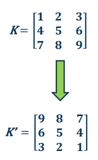
An intuitive interpretation of the relationship:
- Take the kernel, and rotate 180 degrees along center (sometimes referred to as “flip”)
- Perform cross-correlation
- (Just dot-product filter with image!)
Summary: Convolutions are just simple linear operations
So why bother? Why not just call it a linear layer with a small receptive field?
- There is a duality between convolutions and receptive fields during backpropogation
- Convolutions have various mathematical properties people care about (we are those people)
- This is historically how they’ve come about
Input and Output Sizes
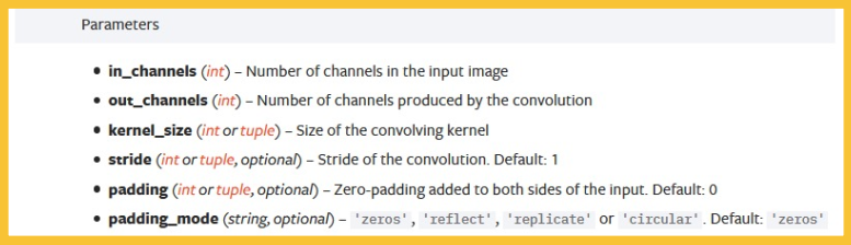
Convolution Layer Hyper-Parameters (PyTorch)
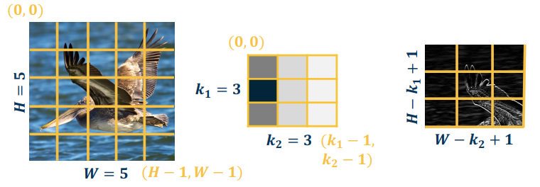
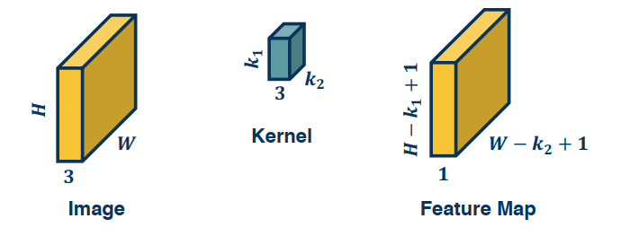
Valid Convolution
Output size of a vanilla convolution operation is $$(H-k_1+1) \times (W-k_2+1)$$.
This is called a “valid convolution” and only applies kernel within image.
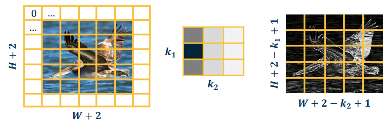
Adding Padding
We can pad the images to make the output the same size:
- Zeros, mirrored image, etc.
- Note padding often refers to pixels added to one size (P=1 here)
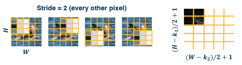
Strides
Strides refers to the movement of the convolution. The default of one means we move the filter one pixel, but we can take larger strides.
- This can potentially result in loss of information
- Can be used for dimensionality reduction (not recommended)
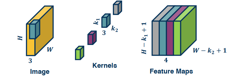
Multi-Channel Inputs
While we have generally spoken of images and kernels as 2 dimensional, this isn’t a hard and fast rule. In fact many of the images we work with have colours, ant t/f must have a third dimension called the channel (which is always 3). The third dimension refers to the RGB structure of the image and would not exist in a greyscale, or black and white, image.
To perform convolutions on such images we simply add a 3rd channel to our convolution kernel, and multiply/copy our kernel across all 3 dimensions. To perform the convolution we again perform elementwise multiplication between the kernel and the image patch, then sum them up like a dot product.
We also can have multiple kernels per layer. In this case, we stack the feature maps together at the output.
Of course we can also vectorize these operations by flattening the image patch as row vectors, then flatten the kernels and take their transpose to produce column vectors.
Pooling Layers
Recall that dimension reduction is an important aspect of Machine learning. How can we make a layer to explicitly down sample an image or feature map? Well the answer is pooling operations!
Parameters needed to Pool:
- Kernel size: Size of window to take the max over
- Stride: the stride of the window. (Default = kernel size)
- Padding: Implicit zero Padding to be added on both sides
Max Pooling
Stride a window across an image and perform per-patch max operation.
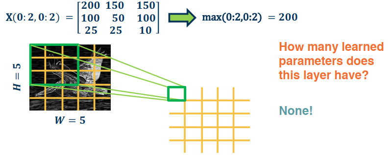
We are not restricted to max either. In fact you can use any differentiable function (average, min, etc etc).
Since the output of convolution and pooling layers are (multi-channel) images, we can sequence them just as any other layer.
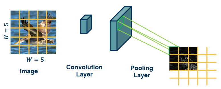
This combination adds some invariance to translation of features. If feature (such as beak) translated a little bit, output values still
remain the same.
Convolution by itself has the property of equivariance. For example, if feature (such as beak) translated a little bit, output values move by the same translation.

