Deep Learning-1-3 Optimization of Deep Neural Networks Overview

Learning Objectives

• Optimization
• Architecture
• Data Consideration
• Training to Optimize
• ML Considerations (Regularization & Overfitting)

---

Overview

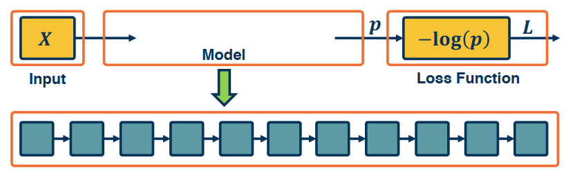
Backpropagation, and automatic differentiation, allows us to optimize any function composed of differentiable blocks.

• There is no need to modify the learning algorithm depdent on what’s inside
• The complexity of the function is only limited by computation and memory

A network with two or more hidden layers is often considered to be a deep model. Depth is important for several reasons:

1. it is needed to structure a model to represent an inherently compositional world. We have object shapes, parts and scenes for example in Computer vision.
2. Theoretical evidence also suggests it leads to parameter efficiency. For example, a two layer NN, you will need exponentially more nodes to learn this function.
3. Gentle dimensionality reduction.

However, there are still many design decisions that must be made:

• How do you architect the mode to reflect the structure
• Data considerations such as normalizations and scaling.
• Training and optimization
• ML consideration; how to optimize through methods such as regularization in order to tame our model.

Architecture

1. What modules or layers should we use?
2. How are they shared, and how should the be connected
3. How will the gradients flow
4. Can they domain knowledge add architectural biases

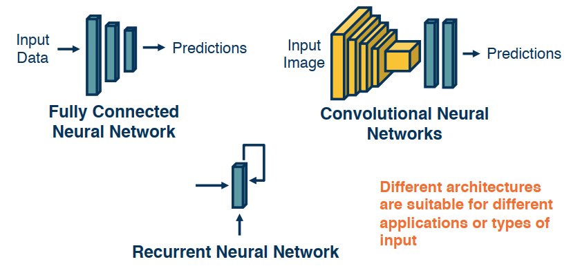
Examples of architectures:

Fully Connect NN

Take an input, convert it to a vector, then feed it into a series of linear and nonlinear transformations. There are be hidden layers in the middle that are expected to extract more and more abstract features from the high dimensional raw input data. For deeper networks we will want to reduce the features/size. In the end we have a layer that represents our class scores. each node will have an outptu that represents a score and these are combined to produce a probability. This is not very good for say images as the number of pixels is generally very high, and it ignores the spatial sctructure of the images. So we turn to CNNs

CNN-Convolutional Neural Networks:

Rather than tie each node to each pixel, these will reflect a feature extractuor for small windows in the image and each local window will have these features extracted from it such as shapes corners, eyes and wheels. In the end we will features that represent where each object or entire objects are located in the image. Finally we will pass these features into a fully connected layer. Albeit this time it will be a much smaller than the previous approach.

RNN-Recurrent Neural Networks:

another approach better suited for problems that have a sequential structure like NLP and sentences.

Data Consideration

As in traditional machine learning, data is key, we will face the questions:

• How do we pre-process
• Should we normaile? or standardize.
• Can we augment our data? would adding noise reflect the real world?

Training and Optimization

Even given a good neural network architecture, we need a good optimization algorithm to find good weights

• What optimizer should we use?
  • We need a good optimization algo to find our weights. Gradient descent is popular but there are others that still use gradients. Different optimizaers may make more sense.
• How do we init our weights?
  • A bad initilization can lead to difficult learning and require a diff optimizer.
• What regularization should we use? How can we prevent overfitting?
• Loss function: which one do we use? do we design our own?

Machine Learning Consideration

The practice of ML is complex. For any application you must look at the trade-offs between the considerations above. Another trade-off is model capacity and the amount of data. Low capacity models can preform poorly when certain loss functions like sigmoid are used.

Unfortunately, all this is done via experience … there is no good text book on all these.

Architecture Considerations

What modules to use, and how to connect them?

• This is guided by the type of data being used and it’s characteristics.
• Lots of data types (modalities) already have good architectures.
• The flow of gradients is the top most consideration when analyzing layers. It is quite possible to have modules that cause a battleneck.
• Combinations of linear and non linear layers.
  • A combo of linear layers only has the same representational power as one linear layer.
  • Non linear layers are crucial. Compositions of nonlinear layers enables complex transformations.
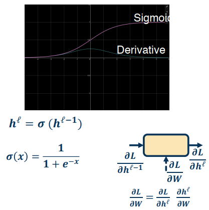
  • Gradient flow depends heavily on the shape of the nonlinear modules.

Several aspects that we can analyze:

• The min/max
• Correspondence between input and output statistics
• Gradients
  • at initialization: are they changing? if so how
  • at the extremes of the function
• Computational complexity

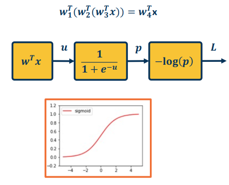
Sigmoid

• Min=0; max=1
• Output is always positive
• Saturates at both ends
• Gradients
  • vanish at each end ( converging to 0 - it’s almost flat )
  • always positive
• Computationally complexity high due to exponential term

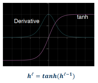
tanh

• min=-1; max=1; and we note that is centred
• Saturates at both ends (-1,1)
• Gradients: vanish at both ends ; always positive
• Medium compexity as tanh is not as simple as say multiplication

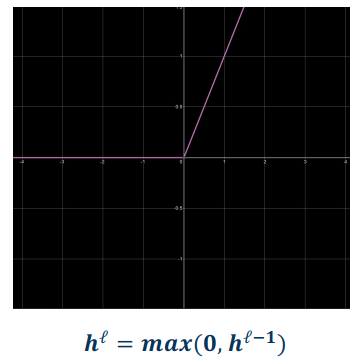
ReLU

• Min=0, Max=infinity
• Output always positive
• Not saturated on the positive side
• Gradients: 0 when X <= 0 (aka dead ReLU); constant otherwise (doesn’t vanish which is good)
• Cheap: doesn’t come much easier than max function

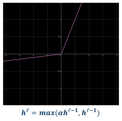
Leaky ReLU

• Min=-infinity, Max=infinity
• Prevents dead ReLU;
• It has a learnable parameter (provides flexibility)
• No saturation on either side
• Still cheap to compute

Selecting a Non-Linearity

Which non-linearity should you select?

• Unfortunately, no one activation function is best for all applications
• ReLU is often the best starting point and is very popular.
  • You may have noticed these are not differentiable. Turns out this is ok because there are few problematic points. only 0 is not differentiable. Converges very quickly.
  • Sometimes a leaky ReLU is a good thing and can make a difference.
• Sigmoid is generally avoided, except in some cases where we need the values to fit the 0-1 range.

Initialization

The parameters of our model must be initialized to something.

Initialization is extremely important!

• Determined how statistics of outputs (given inputs) behave
• Determines how well gradients flow in the beginning of training (important)
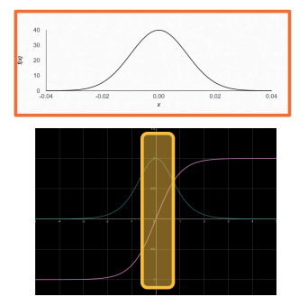
  • If you initialize the weights to values that are in some way degenerate (close to a bad local minima) then this will lead to poor gradient flow.
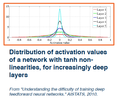
  • If the weights are initialized to be activated into statistically large and these large activations are fed into our nonlinearities (such as the tanh) then the algo will begin in the saturation range of the function.
• Could limit use of full capacity of the model if done improperly

Constant Weights

**Let’s consider an example. What happens when we use constant weights? **

This would lead to a degenerate solution, as all weights will be updated with the same rule. they will move in the same direction and with the same step size. There are cases where this may be good, so it depends.

Small Normally Distributed Random Number

A common approach is to use small normally distributed random number. Eg. $N(\mu=0,\sigma=0.01)$

• Smaller weights are preferred since no feature or input has a priori importance
• Keeps the model within the linear region of most activation functions

Deeper networks (with many layers) are more sensitive to initialization.

• With a deep network, activations (outputs of nodes) get smaller. Standard deviation reduces signficantly.
• This leads to smaller values multiplied by upstream gradients.
• Larger values will lead to saturation. We want a balance between the layers but this proves to be more difficult as complexity increases.

Uniform Distrinution

Ideally, we’d like to maintain the variance at the output to be similar to that of the input. This condition leads to a simple initialization rule, we sample from the uniform distribution:
$$
(-\frac{\sqrt6}{\sqrt {n_j+n_{j+1}}}, +\frac{\sqrt6}{\sqrt{n_j+n_{j+1}}})
$$
Where, $n_j$ is fan-in (number of input nodes), $n_{j+1}$ is fan-out (number of output nodes).

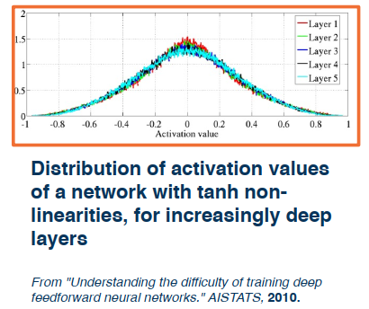
Notice how the distribution is relatively equal across all the layers.

In practice there is an even simpler form,$$N(0,1)*\sqrt{\frac{1}{n_j}}$$, This analysis holds for tanh and similar activations.

For ReLU activations a similar analysis yields: $$N(0,1)*\sqrt{\frac{1}{n_j/2}}$$

Summary

• Initialization Matters
• It determines the activation (output) statistics and therefore gradient statistics
• If gradients are small learning is difficult if not impossible. Vanishing gradients become blockers to learning
• It’s important to reason about output gradient statistics and analyze them for new layers and architectures.

Normalization, Processing, and Augmentation

Data Processing

In ML and DL data drives the learning of features and classifiers.

• Its characteristics are therefore extremely important.
• Always seek to understand your data is important before transforming.
• Relationships between output stats, layers such as non-linearities, and gradients is important.

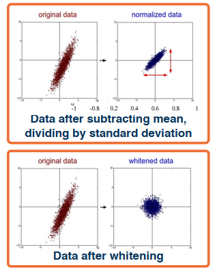
Just like initialization, normalization can improve gradient flow and learning. Typically methods include:

• Subtract the mean, divide by the standard deviation (sometimes a small epsilon is added for numerical stability)
  • can be done per dimension (indepepndently)
• Whitenining methods such as PCA can be used but are not too common

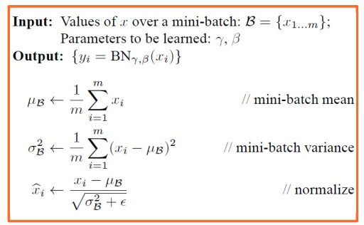
Somtimes we will use a layer that can normalize the data across the neural network. For example:

• Given a minibatch od size BxD where B is the batch size
• Compute the mean and variance for each dimension d in the batch
• Normalize using this mean/variance

This will allow the network to determine it’s scaling, or normalizing, factors, giving it greater flexibility. This is called Batch Normalization. During inference, stored mean and variances calculated on training sets are used. Sufficient batch sizes must be used to get stable per-batch estimates during training.

Batch Normalization presents some interesting challenges: Sufficient batch sizes must be used to get stable per-batch estimates during training.

• This becomes especially true when using multi-GPU or multi-Machine training
• pytorch has a built in function to handle these situations, it estimates the batch statistics in these settings (torch.nn.SyncBatchNorm)

Normalization is especially important before non-linearities. We want the input statistics to be well behaved such that they do not saturate the non-linearities. We do not want too low, or too high, or even unnormalized and unbalanced values, because they cause desaturation issues.

Optimizers

So far we have only talked about Steepest gradient descent, this section introduces other approaches.

Deep learning often involves complex, compositional and nonlinear function. Consequently the loss landscape is often complex as a result. There is little direct theory and a lot of intuition needed to optimize these loss surfaces.

Some Issues

It used to be thought that existence of local minima is the sticking point in optimization. But it turns out this is not always true. In many cases though we can find local minima, but there may be other issues that arise and hinder our ability.

Other issues include

• Noisy gradient estimates (due to taking MiniBatches)
• Saddle points
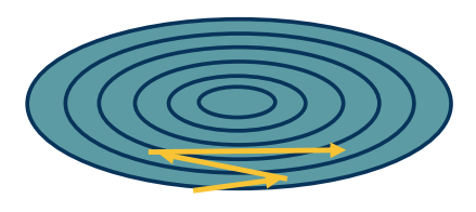
• III conditioned loss surface, where the curvature is high in one direction but not the other

We generally use a subset of the data in each iteration to calulate the loss and the gradient. This is an unbiased estimator, but can have high variance.

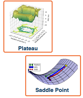
Several loss surface geometries can present difficulties for optimization:

• Several types of minima: local minima, plateaus, saddle points
• Saddles points are those where the gradient of orthogonal directions are zero

Momentum

Steepest gradient descent is always searching for the steepest direction, and can become stuck at saddle points. One way to overcome this is to think of momentum. Imagine a ball rolling down a loss surface, and use momentum to pass flat surfaces.

Recall our update rule from earlier:
$$
w_i=w_{i-1}-\alpha\frac{\partial L}{\partial w_i}
$$
Consider update velocity (starts as 0, $\beta = 0.99$):
$$
v_i=\beta v_{i-1}+ \frac{\partial L}{\partial w_{i-1}}
$$

Our new update rule:
$$
w_i=w_{i-1}-\alpha v_i
$$

Note that when $\beat=0$, this is just Stochastic Gradient Descent (SGD)

This is acutally used quite often in practice, and can help move you off areas with low gradients. Observe that the velocity term is an exponential moving average of the gradient.

$$
v_i = \beta v_{i-1} + \frac{\partial L}{\partial w_{i-1}}\
= \beta (\beta v_{i-2} + \frac{\partial L}{\partial w_{i-2}}) + \frac{\partial L}{\partial w_{i-1}}\
= \beta^2v_{i-2} + \beta \frac{\partial L}{\partial w_{i-2}} + \frac{\partial L}{\partial w_{i-1}}
$$

This is actually part of a general class of accelerated gradient methods with theoretical analysis under some assumptions.

Nesterov Momentum

Nesterov Momentum: Rather than combining velocity with the current gradient, go along velocity first and then calculate the gradient at a new point.

$$
\widehat{w_{i-1}}=w_{i-1}+\beta v_{i-1}\
v_i=\beta v_{i-1} + \frac{\partial L}{\partial \widehat{w_{i-1}}}\
w_i=w_{i-1} - \alpha v_i
$$

Of course there are various equivalent implementation, should you choose to google this you’ll find a few.

Hessian and Loss Curvature

There are various mathematical ways to characterize the loss curve. Similar to Jacobians, Hessians use 2nd order derivatives that provide further information about the loss surface.

However, these are computationally intensive. The ratio between the smallest and largest eigenvalue of a hessian is called a condition number. Condition Numbers tell us how different the curvature is along different dimensions.

If it is high then SGD (Stichastic Gradient Descent) will make big steps in some dimensions and small steps in others. This will cause a lot of jumping and learning becomes sporadic and unpredictable.

There are other second order optimization methods that divide steps by curvature, but are expensive to compute.

Pre-Parameter Learning Rate

Idea here is to have a dynamic learning rate for each weight.

Several flavors of optimization Algorithms:

• RMSProp
• Adagrad
• Adam
• …

There is no one method that is the best in all cases. While SGD can achieve similar results it’ll require much more tuning.

Adagrad

Adaptive Subgradient Methods for Online Learning and Stochastic Optimization.

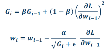
Idea: Use gradient statistics to reduce learning rate across iterations.

This method uses a gradient accumulator $G_i$:
$$
G_i=G_{i-1}+(\frac{\partial L}{\partial w_{i-1}})^2\
w_i=w_{i-1}-\frac{\alpha}{\sqrt{G_i+\epsilon}}\frac{\partial L}{\partial w_{i-1}}
$$

Directions with high curvature will have higher gradients, and learning rate will reduce.

RMSProp

One shortcoming to Adagrad is that the accumulator continues to grow, meaning that the denominator grows large, which will push the learning rate towards 0. So what do we do? Well we can apply the idea of a weighted/moving average rather than a simple additive accumulator.

Adam

Another Approach that is very popular is Adam, and combines aspects from both of the above.

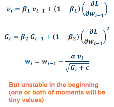
One drawback is that this performs poorly near small values, and can become instable. So we apply a Time Varying bias, to get the version that is used most often in practice.

Behavior of Optimizers

It’s important to note that all these optimizers act differently depending on the loss landscape/sruface.

They will exhibit different behaviours such as overshooting, Stagnating, etc.

Plain SGD+Momentim can generalize better than adaptive methods but require more tuning.

Learning Rate Schedules

First order optimization methods use learning rate. Theoretical results rely on annealed learning rate.

Several Typical Schedules:

• Graduate Student GD - By Observation
• Step scheduler - Reduce the learning rate every n epochs
• Exponential scheduler
• Cosine Scheduler - Learning rate decays according to a cosine drive function

Regularization

This is a crucial aspect needed in DL as well as ML. Some examples are:

1. L1 Norm - Penalizes Large weights and encourages sparsity and smaller weights
   $$
   L=|y-Wx_i|^2+\lambda |W|
   $$
2. L2 Norm - Behaves similar to the L1 but it does so in a different way
   $$
   L=|y-Wx_i|^2+\lambda |W|^2
   $$
3. Elastic L1/L2:
   $$
   L=|y-Wx_i|^2+\alpha |W|^2 + \beta |W|
   $$

Dropout Regularization

A problem that is commonly encountered is that a Network often will learn to rely heavily on a few strong features that work very well. This often results in overfitting as the model is not representative of the data.

To prevent this we employ drop-out regularization: For each node, keep it’s output with probability p. Activations of deactivated nodes are essentially zero. This can mask out a particular node in each iteration. In practice this can be done by implementing a mask calculated at each iteration.

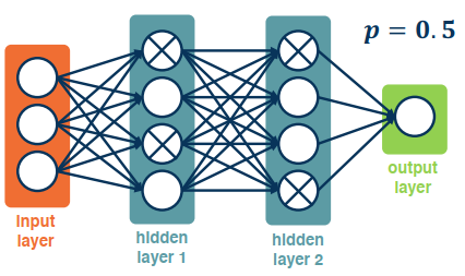
• During training, each node has an expected $𝒑 * 𝒇𝒂𝒏_𝒊𝒏$ nodes.
• During testing you wouldn’t want to drop any nodes. All nodes are activated.
• This violates a basic principle in model building, namely the training and testing data should have similar input/output distributions.

Solutions
During test time, scale outputs (or equivalently weights) by 𝒑

• i.e. $W_{test}=pW$
• Alternatively we could scale by 1/p at training time

Why does this work?

• The model should not relay too heavily on a particular feature
  • If it does it has probability (1-p) of losing that feature in an iteration
• Training $2^n$ network
  • Each configuration is a network
  • Most are trained with 1 or 2 mini-batches of data

Data Augmentation

In this section we will look at Data Augmentation techniques to prevent overfitting. The idea is simple: we apply a series of transformations to the data. This is essentially free, and increases the data. Of course we must not change the data, or it’s meaning. ie flipping an image is fine. We want a range of tranformation that mirror what happens in the real world. What about a random crop of an image? This is also fine as it mirrors the real world, we’ve reduced the data but we haven’t really changed it. In fact using this technique might also increase the robustness of your model. Another method similar to this is cut-mix where portions of an image are cut out.

A more sophistated approach is color jitter, performed by adding/subtracting from the values in the red, green, or blue channels. Other transforms include, Translation, Rotation, Scale, Shearing. Of course you can also mix and combine these different techniques. These transforms server to increase your dataset using manipulations of the original.

Another (oddly named) approach is the CowMix variation. This is when an image is masked with a cow hide pattern and then some noise is added. The noise is optional as you can also use the mask to blend two im

The Process of Training Neural Networks

Let’s now turn our attention to the training and monitoring of our Neural Network.

• Trianing deep neural networks is an art form
• Lots of things matter (together). The key is to find a combination that works
• Key Principle: Monitoring everything to understand what is going on!
  • Loss and accuracy curves
  • Gradient statistics/characterisitcs
  • Other aspects of computation graphs

Proper Methodology

Analyzing what is happening always begin with good methodology.

• Separate your data into: Training, Validation, Test set
  • Never look at the test data until the training is complete
  • Meaning your hyperparameters and all other considerations should be locked down
• Use Cross Validation to decide on hyperparameters if the amount of data is an issue

Sanity Checking

Check the bounds of your loss function

• E.g. Cross entropy should be within [0,∞]

• Check initial loss at small random weight values

  • E.g. −log(p) for cross entropy where p=0.5

• Start without regularization and check to see that the loss goes up when added

• Key Principle: Simplify the dataset to make sure your model can properly (over)-fit before appyling regularization
  small datasets can easily be fit - if this doesn’t happen then your model is bad

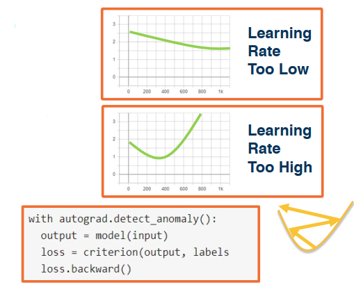
Loss and Not a Number (NaN)

Change of loss is indicative of the rate/speed of learning. Always plot and monitor learning curves: Iterations v.s. Loss. This reveals issues:

1. A tiny loss change implies too small of a learning rate.
   • It might still converge but you’ll be waiting a while
2. Loss (and then weights) turn to NaNs imply too high of a learning rate.
   • This results in a learning rate resembling a quadratic function
   • Might indicating bouncing away from a local minima
   • This may also be caused by division by 0, so be careful.

Overfitting

Of course classic machine learning signs of under/over fitting still apply!

• Over Fitting: Validation loss/accuracy starts to get worse after a while. In other words, gap between training and held out data is increasing
• Under Fitting: Validation loss very close to training loss, or both are high. Training set performance is poor and model is simply not very powerful.
• Note: You can have higher training loss than validation loss
  • Validation loss has no regularization, this can be problematic
  • Validation loss is typically measured at the end of an epoch

Hyper-Parameter Tuning

Lots of hyperparamters to tune (NB the weights are NOT hyperparamters). Hyperparameters gen refer to the more design decisions that go into the construction of the network.

• Learning Rate, Weight Decay, are crucial
• Momentum
• Number of layers and number of nodes

Even a good idea will fail if not tuned properly!

Typically you should start with a coarse search:

• ie {0.1, 0.05, 0.03, 0.01, 0.003, 0.001, 0.0005, 0.0001}
• Then perform a finer search around the values that perform well

There are automated methods that are decent, but intuition (and even randomness) can do well given enough of a tuning budget.

Interdependence of Hyperparameters can be troublesome! Examples:

• Batch Norm and drop out are often not needed together, they can make things even worse!
• Learning rate should be proproptional to batch size. Increase the learning rate for larger batch sizes
  • Gradients are more reliable and smoother

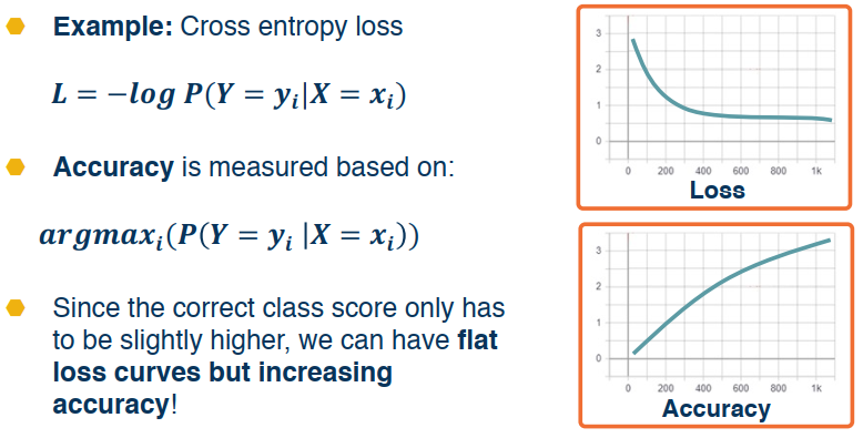
Relationship Between Loss and Other Metrics

Remember that DL we are optimizing a loss function that is differentiable. However what we care about are the metrics surrounding the model which we cannot optimize (lack of derivatives).

• Accuracy
• Precision & Recall
• Other specialized metrics

The relationship between these and the loss curve can be complex!

Here’s another example that looks at True Positive Recall (TPR) & False Positive Recall (FPR)

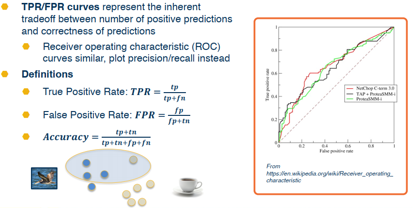
Finally we can obtain a curve by varying the probability threshold. The area under the curve (AUC) is a common single number metric used to summarize.

Mapping between these and the loss however is not so simple or straight forward.