Deep Learning-1-2 Neural Networks

Learning Objectives

• NN vie as Linear Classifiers
• Computation Graphs
• Backpropagation
• Backprop via AutoDiff
• DAG Logistic Regression (Sigmoid)
• Simple Layer Jacobians and Vectorization

---

NN view as Linear Classifiers

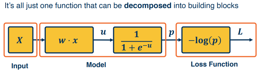
A linear classifier can be broken down into: 1) input; 2) A function of the inputs; 3) A loss function.

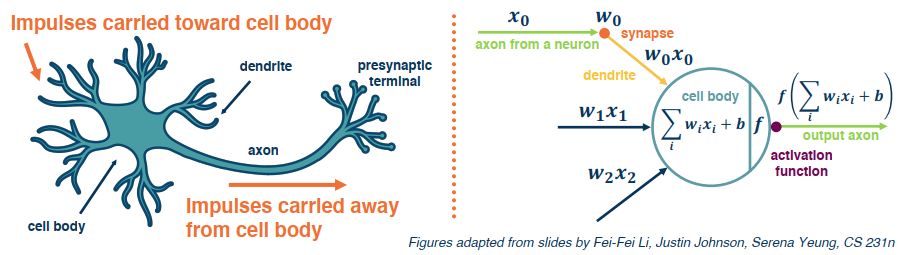
A simple neural network has similar structure as our linear classifier:

1. A neuron takes input (firings) from other neurons (-> input to linear classifier)
2. The inputs are summed in a weighted manner (-> weighted sum/dot product)
3. Learning is through a modification of the weights (application of the update rule)
4. If it receives enough input, it “fires” (threshold or if weighted sum plus bias is high enough)

Of course this is an oversimplified model of the neurons in our brain.

We can also have many neurons connected to the same input. This is what happens in a multi-class classifier. Each output node outputs the score for a class. These are often call “fully connected layers”, or linear projection layers.

$$
f(x,W)=\sigma(Wx+b) \begin{bmatrix}
w_{11} & w_{12} & … & w_{1n}\\
w_{21} & w_{22} & … & w_{2n}\\
…\\
w_{m1} & w_{m2} & … & w_{mn}\\
\end{bmatrix}
$$

Computation graph

A nice illustration by colah’s blog can help better understand.

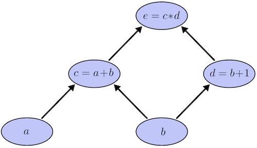
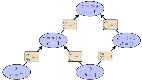
Computational graphs are a nice way to think about mathematical expressions. For example, consider the expression e=(a+b)∗(b+1). There are three operations: two additions and one multiplication. To help us talk about this, let’s introduce two intermediary variables, c and d so that every function’s output has a variable. We now have:

c=a+b
d=b+1
e=c∗d

To create a computational graph, we make each of these operations, along with the input variables, into nodes. When one node’s value is the input to another node, an arrow goes from one to another.

Derivatives with Computation Graph

If one wants to understand derivatives in a computational graph, the key is to understand derivatives on the edges. If a directly affects c, then we want to know how it affects c. If a changes a little bit, how does c change? We call this the partial derivative of c with respect to a.

Logistic Regression Gradient Descent

Logistic Regression on m Examples

The cost function is computed as an average of the $m$ individual loss values, the gradient with respect to each parameter should also be calculated as the mean of the $m$ gradient values on each example.

The calculattion process can be done in a loop through m examples.

J=0
dw=np.zeros(n)
db=0

for i in range(m):
  z[i] = w.transpose() * x[i] + b
  a[i] = sigmoid(z[i])
  J = J + (-[y[i]*log(a[i])+(1-y[i])*log(1-a[i])])
  dz[i] = a[i] - y[i]
  
  # inner loop for n features, later will be optimized by vectorization
  for j in range(n):
    dw[j] = dw[j] + x[i][j] * dz[i]
  
  db = db + dz[i]
  
j = j / m
dw = dw / m
db = db / m

After gradient computation, we can update parameters with a learning rate alpha.

# vectorization should also applied here
for j in range(n):
  w[j] = w[j] - alpha * dw[j]
b = b - alpha * db

As you can see above, to update parameters one step, we have to go throught all the m examples.

Backpropagation

Backpropagation algorithm consists of two main parts:

1. Forward pass - which computes the outputs for a given set of weights
2. Backward pass - calculates the gradients for each module, can be decomposed into several steps:

• This is a recursive algorithm
• Start at the loss function where we know how to compute the gradients
• Progress backwards throught the modules (computing the gradients at each stage)
• Ends at the input layer where there are no gradients or parameters

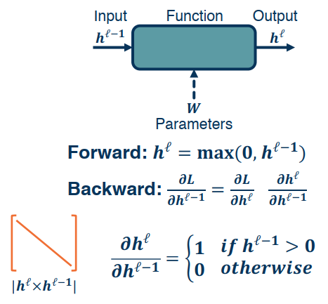
Forward Pass

We simply compute the output of each component and save. These will be needed to compute the gradients later on.

Backwards Pass

It is much more complex and involved, recursive algorithm. Here we seek to calculate the gradients of the loss with respect to the module’s parameters.

There are three main gradients needed for each module:

1. $\frac{\partial L}{\partial h^{l-1}}$ is the gradient of the input layer (previous)
2. $\frac{\partial L}{\partial h^{l}}$ is the gradients of the output layer (current)
3. $\frac{\partial L}{\partial W}$ is given to us by the forward pass

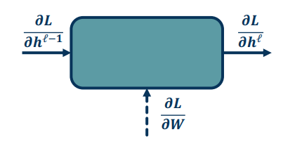
We need to compute the local gradients:
a. $\frac{\partial h^l}{\partial h^{l-1}}$ – The change in the output with respect to the inputs

b. $\frac{\partial h^l}{\partial W}$ – The change in the putput wrt the weights

c. $\frac{\partial L}{\partial h^{l-1}}$

d. $\frac{\partial L}{\partial W}$

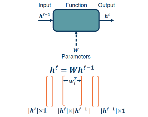
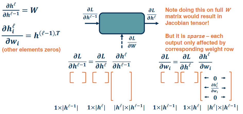
Compute local gradients $\frac{\partial h^l}{\partial h^{l-1}}$ and $\frac{\partial h^l}{\partial W}$

This is simply the derivative of the function wrt it’s parameters and inputs.
For example in a single network $h^l=Wh^{l−1}$
$\frac{\partial h^l}{\partial h^{l-1}} = W$ and $\frac{\partial h^l}{\partial W}=h^{l-1,T}$

Compute $\frac{\partial L}{\partial h^{l-1}}$ and $\frac{\partial L}{\partial W}$

We simply apply chain rule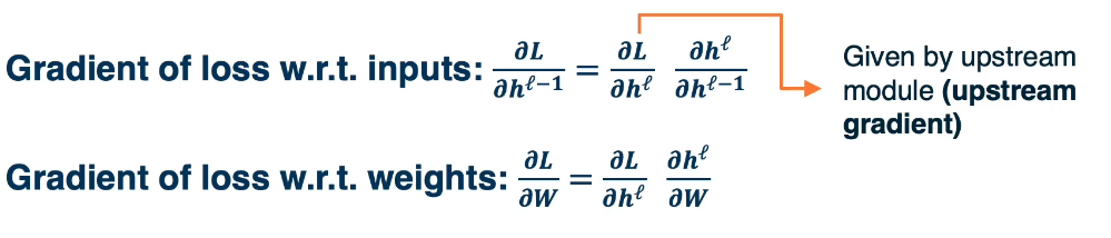

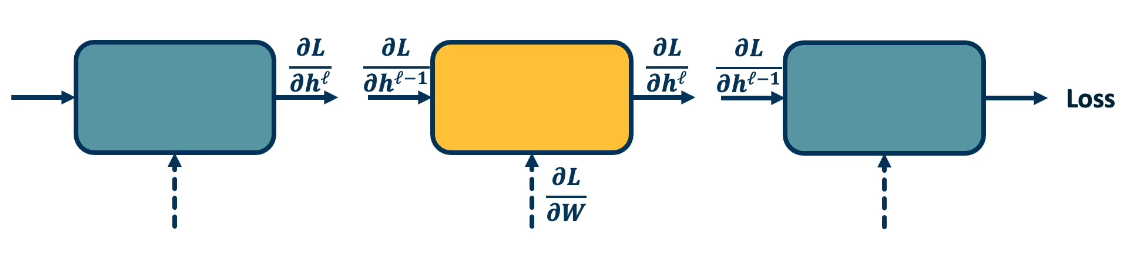
Summary

1. Forward Pass: Compute the Loss on a Minibatch
2. Backward Pass: Compute the gradients wrt each parameter

• Starting at the loss function, where we know how to compute the gradient of the loss wrt the last module
• This is just the partials of the module wrt the inputs
• Now we continue to work backwards propogating the loss in reverse (Upstream)
• This is done using the chain rule

3. Finally we just update the weights
   $$
   w_i=w_i-\alpha \frac{\partial L}{\partial w_i}
   $$

Backprop via AutoDiff

Backprop only tells you what you need to do, it doesn’t specify how to do it. The backprop idea though can be applied to any directed acyclic graph, aka DAG. Graphs represent an ordering constraining which paths must be calculated first. Given an ordering, we can then iterate from the last module backwards, using the chain rule. As we do so we will store it’s gradient outputs for efficient computation. This is called reverse mode automatic differentiation.

The idea here is that we need to create a framework such that we can just define the computation graph. We can put together a set of functions that use simple primitives like addition and multiplication etc etc. Doing so will allow us to avoid computing the backwards gradients, nor will we write code that computes the gradients of the functions. Because these are all simple primitives.

Terminology

1. Computation = Graph

• Input = Data + Parameters
• Output = Loss
• Scheduling = Topological ordering

2. Auto-Diff

• A family of algorithms for implementing chain rule on computation graphs

Examples

We want to find the partial derivative of the output $f$, with respect to all the intermediate variables.

For convenience we assign intermediate variable with a simplify notation. Denote bar as:
$$
\overline{a_3}=\frac{\partial f}{\partial a_3}
$$

We start at the end and work backwards.

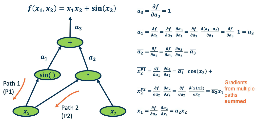
It is interesting to note what certain operations do, and what they tell us about gradient flow.

1. Addition operation distributes gradients along all the paths. e.g. $\overline{a_3}=\overline{a_1}$ and also $\overline{a_3}=\overline{a_2}$.
2. Multiplication operation is a gradient switcher (multiplies it by the values of the other term). e.g. $\overline{x_2}=\overline{a_2}x_1$, and $\overline{x_1}=\overline{a_2}x_2$
3. In Max operation, gradient flows along the path selected to be the max

Key Idea is to store the computation graph in memory and corresponding gradient functions.
Nodes broken down to basic primitive computations (addition, multiplication, log, etc.) for which corresponding derivative is known.

Here’s a small example demonstrating graph building using pytorch: (This uses an older version of pytorch, it’s easier today)

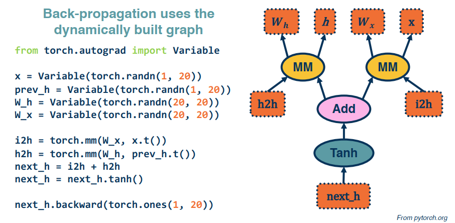
The last line computes the backwards gradients. All in one line of code.
Computation graphs are not limited to mathematical functions. They can have control flows (if’s, loops, etc etc) and can proprogate through algorithms. Also, they can be done dynamically so that gradients are computed, nodes are added, and repeat. All this falls under the umbrella of differentiable programming.

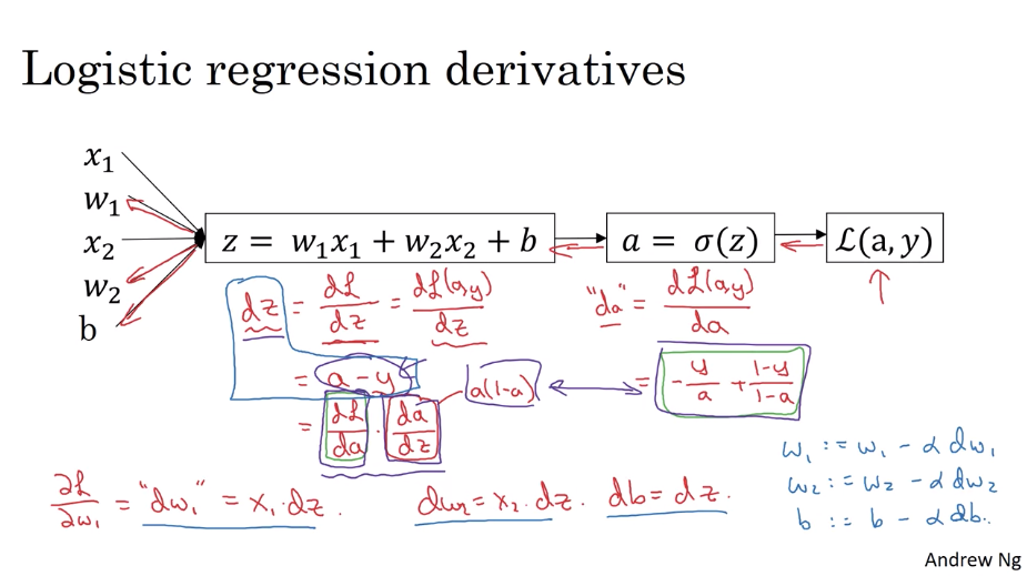
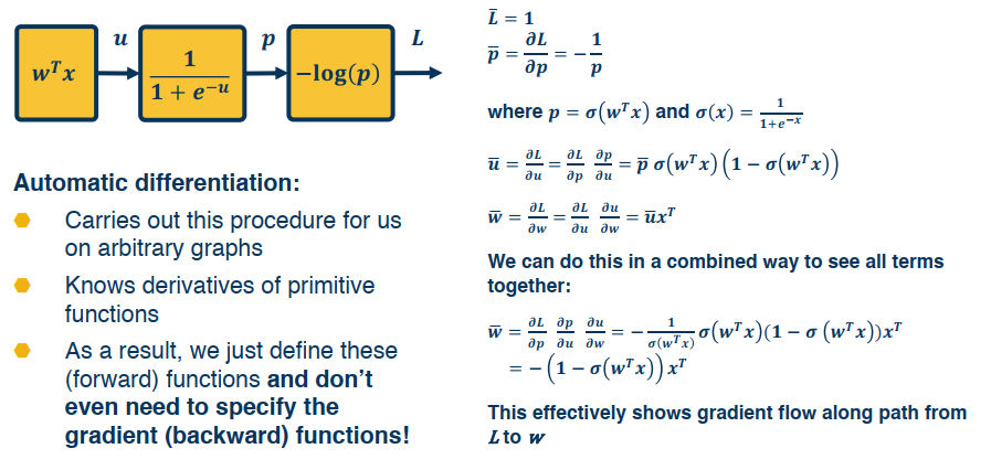
DAG Logistic Regression (Sigmoid)

In this section we look an example that more closely resemble a NN use case. Recall from our earlier sections the sigmoid function given by the Logistic regression function.
$$
-log(\frac{1}{1+e^{-w^Tx}})
$$
where, input $x \in \mathbb{R^D}$, binary label $y \in {-1,1}$, parameters $w \in \mathbb{R^D}$, output prediction $p(y=1|x)=\frac{1}{1+e^{-w^Tx}}$, loss $L=\frac{1}{2}||w||^2-\lambda log(p(y|x))$.

It can be decomposed as follow:

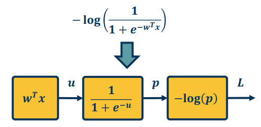
Now, let’s work through the backprop via automatic differentiation.

Vectorization and Jacobians of Simple Layers

Vectorization

Both GPU and CPU have parallelization instructions. They’re sometimes called SIMD instructions, which stands for a single instruction multiple data. The rule of thumb to remember is whenever possible avoid using explicit for loops.

Vectorizing Logistic Regression

If we stack all the $m$ examples of $x$ we have a input matrix $X$ with each column representing an example. So by the builtin vectorization of numpy we can simplify the above gradient descent calculation with a few lines of code which can boost the computational efficiency definitely.

Z = np.dot(w.T, X) + b
A = sigmoid(Z)
dz = A - Y

# in constrast to the inner loop above, vectorization is used here to boost computation
dw = 1/m * np.dot(X, dz.T)
db = 1/m * np.sum(dz)  

Update parameters:

w = w - alpha * dw
b = b - alpha * db

Simple Layer Jacobians and Vectorization

Let’s reconsider our computation graph using matrix notation:

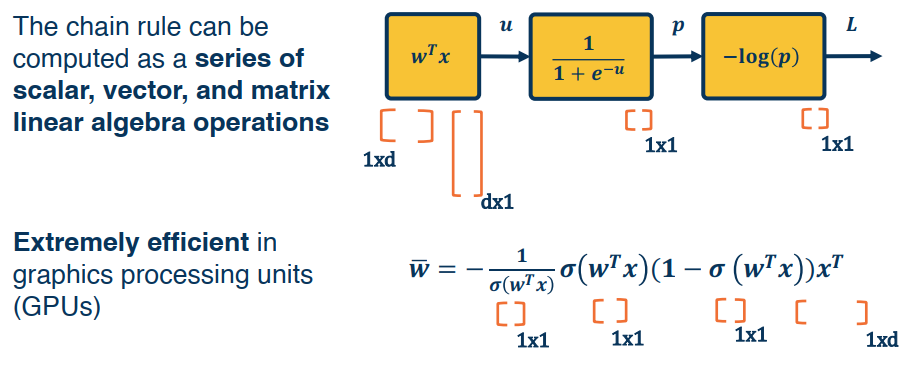
For a simple layer network $h^l=Wh^{l-1}$, $h^l$ has the dimension of $|h^l|\times 1$, $W$ has the dimention of $|h^l|\times |h^{l-1}|$, and $h^{l-1}$ has the dimension of $|h^{l-1}|\times 1$.

Now let’s dive into partials (Jacobians).

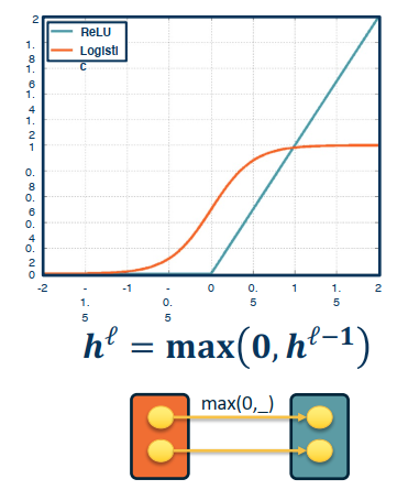
Up until now we’ve focused mostly on our sigmoid function, but we can use any differentiable function! This includes piesewise differentiable functions as well.

A popular choice in many applications is the ReLU (Rectified Linear Unit)
$$h^l=max(0,h^{l-1})$$
It provides non-linearity but better gradient flow than sigmoid, and is performed element wise.

Full Jacobian of ReLU layer is large (output dim x input dim).

• But it is sparse
• Only diagonal values non-zero, because it is element-wise
• An output value affected only by corresponding input value

Recall that Max() function funnels gradients through selected path. Gradient will be zero if input <= 0.