Learning Objectives
- What is neural network?
- Supervised Learning
- Parametric Learning
- Performance Measurement
- Linear Algebra Review
- DL v ML differences
- Logistic Regression and Gradient Descent
What is neural network?
Neural network is a powerful learning algorithm inspired by how the brain works. The definition from mathworks is as follow:
A neural network (also called an artificial neural network) is an adaptive system that learns by using interconnected nodes or neurons in a layered structure that resembles a human brain. A neural network can learn from data—so it can be trained to recognize patterns, classify data, and forecast future events.
A neural network breaks down the input into layers of abstraction. It can be trained using many examples to recognize patterns in speech or images, for example, just as the human brain does. Its behavior is defined by the way its individual elements are connected and by the strength, or weights, of those connections. These weights are automatically adjusted during training according to a specified learning rule until the artificial neural network performs the desired task correctly.
A neural network combines several processing layers, using simple elements operating in parallel and inspired by biological nervous systems. It consists of an input layer, one or more hidden layers, and an output layer. In each layer there are several nodes, or neurons, with each layer using the output of the previous layer as its input, so neurons interconnect the different layers. Each neuron typically has weights that are adjusted during the learning process, and as the weight decreases or increases, it changes the strength of the signal of that neuron.

Supervised Learning
In supervised learning, we are given a data set and already know what our correct output should look like, having the idea that there is a relationship between the input and the output.
Supervised learning problems are categorized into “regression” and “classification” problems. In a regression problem, we are trying to predict results within a continuous output, meaning that we are trying to map input variables to some continuous function. In a classification problem, we are instead trying to predict results in a discrete output. In other words, we are trying to map input variables into discrete categories.
Examples of supervised learning applications:
| Input (X) | Outout (y) | Application |
|---|---|---|
| Home features | Price | Real estate |
| Ad, user info | Click on ad? (0/1) | Online advertising |
| Image | Object | Photo taging |
| Audio | Test transcript | Speech recognition |
| English | Chinese | Machine translation |
| Image, Radar info | Position of other cars | Autonomous driving |
Structured vs. unstructured data
- Structured data is highly specific and is stored in a predefined format
- Unstructured data is a compilation of many varied types of data that are stored in their native formats
Why is deep learning taking off?
Deep learning is taking off due to a large amount of data available through the digitization of the society, faster computation and innovation in the development of neural network algorithm.
Two things have to be considered to get to the high level of performance:
- Being able to train a big enough neural network
- Huge amount of labeled data
Parametric Learning
Supervised learning can be NonParametric Model which have no explicit mathematical formula, examples of this include decision trees and Knn classifiers. They can also be parametric, which have an explicit formula, examples include logistic regression and neural networks. Linear Classifiers fall into the parametric umbrella. These can face challenges though as the number of dimensions increases.
Let’s now dive deeper into parametric learning algorithms.
Components: 1. Input (Representation) 2. Functional Form of the model (Including parameters) 3. Performance measure to improve (Loss, or objective, function) 4. Algorithm for finding the best parameters (Optimization Algorithm)
Function form: $f(x,w)=y$, where f is the classifier, x is the input vector, w is the weights, y is the output.
One of the simplest example of this is the equation of a line $y=mx+b$. If the output is continuous then we can apply a secondary function in order to turn it into a Binary classifier.
$$f(x)=
\begin{cases}
0& f(x,w)>0\\
1& Otherwise
\end{cases}$$
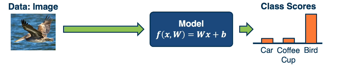
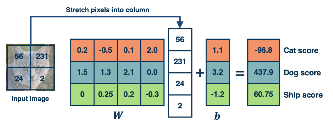
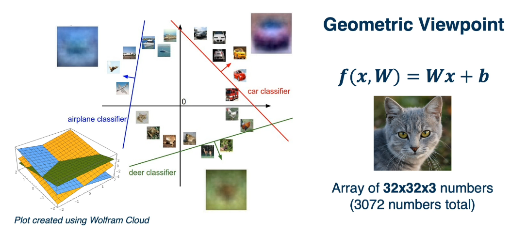
For a multi-class classifier we take the class with the highest (max) score: $f(x,W)=Wx+b$, where W is a matrix and each row represents a class.
Linear Classifiers are models that try to find a line, or hyperplane, that can seperate the data elements into distinct groups. While simple they’re highly versatile and have many applications. However, in order to compute them we will often require a higher dimension and this presents some difficulties.
For more complex functions like XOR and Circles it becomes more difficult, if not impossible to discover a linear seperation. For this we will need none linear activators.
Performance Measurement
Performance Measure to improve the loss or score function. For binary we could take 1 when the score is greater than one and for a multi-class we could take the maximum. However scores suffer from some issues. Difficult to interpret, no bounds and hard to compare to other classifiers. To remedy some of these issues we will use the softmax function to turn scores into probabilities.
For a score function of the form $s=f(x,W)$, we would take the following softmax function to calculate the probability for each class K
$$P(Y=k|X=x)=\frac{e^{s_k}}{\sum_je^{s_j}}$$
In order to optimize this we need a function to optimize. This is often called our loss or objective function. It should have the following properties:
- Penalize model for being wrong
- Allows modification (so we can reduce the penalty)
In ML we will often use empirical risk minimization: Reduce the loss over the training dataset, then average the loss over the training data.
Given${(x_i,y_i)}_{i=1}^N$, we can define the loss as
$$
L=\frac{1}{N}\sum L_i(f(x_i,W), y_i)
$$
where, $x_i$ is an image and $y_i$ is a label (usually an integer).
Consider the example of Support Vector Machines (SVMs), the SVM loss has the form:
$$
L_i=\sum_{j\neq y_i}
\begin{cases}
0& if s_{yi}\geq s_j + 1\\
s_j-s_{yi} + 1& Otherwise
\end{cases}\\
=\sum_{j\neq y_i}max(0,s_j-s_{yi} + 1)
$$
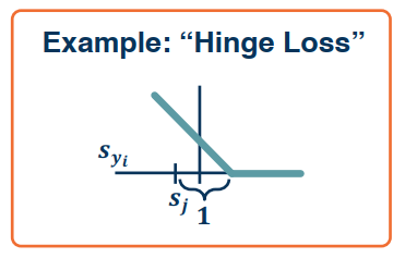
We want to have a score that is higher by some margin for the ground truth label. When this is not the case we penalize this by how different it is from the margin. To do thie we take the max over all the classes that are not the ground truth, and penalize the model whenever the score for the ground truth itself is not bigger by a particular margin. This is called a hinge loss.
Simple example, suppose we are trying to classify a picture into 1 of three categories: cat, frog, or car.
1 | Picture 1 : Ground truth : CAT |
If we use the softmax function to convert scores to probabilities, the following loss function to use is cross-entropy:
$$
L_i=-log P(Y=y_i|X=x_i)
$$
It can be derived by looking at the distance between two probability distributions and also could be derived from a maxim likehood estimation perspective. Maximum Likelihood Estimation: choose the probabilities to maximize the likelihood of the observerd data.
Let’s re-examine our example above using the cross entropy
1 | Recall the ground truth is CAT |
If we are performing regression, we can directly optimize to match the ground truth value.
Example of house price prediction
$L_i=|y-Wx_i|$ – is the L1 loss
$L_i=|y-Wx_i|^2$ – is the L2 loss
For probabilities:
$L_i=|y-Wx_i|=\frac{e^{s_k}}{\sum_je^{s_j}}$ – is Logistic
In some cases we add a regularization term to the loss function to encourage smaller weights, and penalize higher weights which would over emphasis a feature.
$L_i=|y-Wx_i|+|W|$ – is an L1 regularized loss function
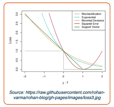
The illustration above shows the characteristics of different loss functions.
Linear Algebra Review
In general we will be working with Matrices W, and X. Where x is the vector.
Size of W, X, and x
- Let $c$ be the number of classes, or targets, and $d$ be the dimensionality, or number of features.
- W is the size of ($c, d+1$), here we add 1 for the bias term
- x is a row vector of size $d+1$
For our discussion, assume s is a scalar $s \in \mathbb{R}^1$, v is a vector $v \in \mathbb{R}^m$, and M is a matrix $M \in \mathbb{R}^{k \times 1}$, then
$\frac{\partial v}{\partial s}$ is of size $\mathbb{R}^{m \times 1}$
$\frac{\partial s}{\partial v}$ is of size $\mathbb{R}^{1 \times m}$
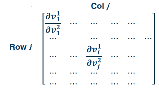
$\frac{\partial v_1}{\partial v_2}$ is of size $\mathbb{R}^{m \times m}$ This is a Jacobian matrix shown as follow.
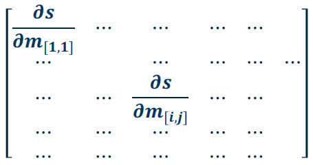
What is the size of $\frac{\partial s}{\partial M}$?
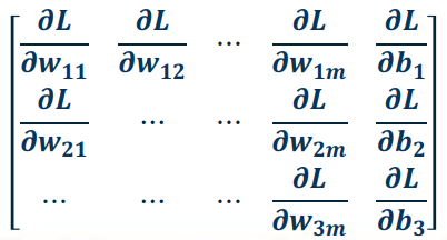
What is the size of $\frac{\partial L}{\partial W}$? By the previous question this should result in a matrix of partials (Jacobian).
Often times our algorithms (like gradient descent) are implemented in batches, which can also be thought of as matrices and tensors.
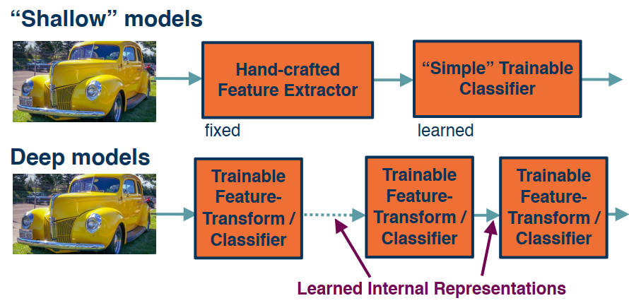
DL vs ML
Deep Learning employs a few key concepts generally expects raw data and learns a feature representation. Neural Networks are the most popular form but there are a few others like probabilistic learning.
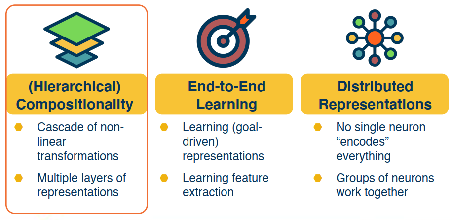
“Shallow” vs. Deep Learning
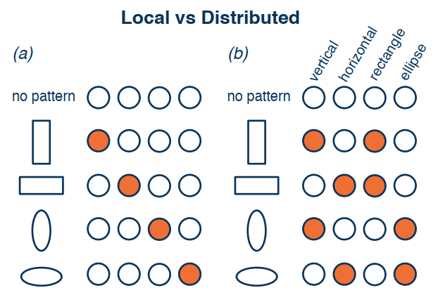
Distributed Representation
Recall that: 1) No single neuron encodes everything; 2) Groups of neurons need to work together
- Local representation: a concept is represented by a single node.
- Distributed representation: a concept is represented by the pattern of activation across many nodes.
Logistic Regression and Gradient Descent
Logistic Regression
Logistic regression is useful for situations in which you want to be able to predict the presence or absence of a characteristic or outcome based on values of a set of predictor variables. It is similar to a linear regression model but is suited to models where the dependent variable is dichotomous. Logistic regression coefficients can be used to estimate odds ratios for each of the independent variables in the model. Logistic regression is applicable to a broader range of research situations than discriminant analysis. (from ibm knowledge center)
A detailed guide on Logistic Regression for Machine Learning by Jason Brownlee is the best summary of this topic for data science engineers.
Andrew Ng’s course on Logistic Regression focuses more on LR as the simplest neural network, as its programming implementation is a good starting point for the deep neural networks that will be covered later.
Logistic Regression Cost Function
In Logistic regression, we want to train the parameters $w$ and $b$, we need to define a cost function.
$$\widehat{y}^{(i)}=\sigma(w^Tx^{(i)}+b)$$,
where $$\sigma(z^{(i)})=\frac{1}{1+e^{-z^{(i)}}}$$
Given ${(x^{(1)},y^{(1)}),…, x^{(m)},y^{(m)})}$, we want $\widehat{y}^{(i)}\approx y^{(i)}$
The loss function measures the difference between the prediction $\widehat{y}^{(i)}$ and the desired output $y^{(i)}$. In other words, the loss function computes the error for a single training example.
$$L(\widehat{y}^{(i)}, y^{(i)}) = -(y^{(i)}*log(y^{(i)}) + (1-y^{(i)})*log(1-y^{(i)}))$$
So,
$$
L(\widehat{y}^{(i)}, y^{(i)}) = \begin{cases}
-log(y^{(i)})& if\ \ y = 1\\
-log(1-y^{(i)})& if\ \ y = 0
\end{cases}
$$
The cost function is the average of the loss function of the entire training set. We are going to find the parameters $w$ and $b$ that minimize the overall cost function.
$$
J(w,b) = \frac{1}{m}\sum_{i=1}^{m}L(\widehat{y}^{(i)}, y^{(i)})\\
= -\frac{1}{m}[\sum_{i=1}^{m}y^{(i)}log(y^{(i)}) + (1-y^{(i)})log(1-y^{(i)}))]
$$
The loss function measures how well the model is doing on the single training example, whereas the cost function measures how well the parameters $w$ and $b$ are doing on the entire training set.
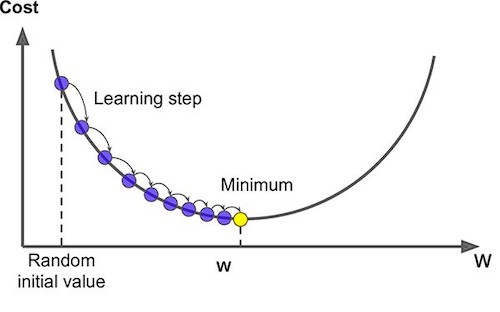
Gradient Descent
As you go through any course on machine learning or deep learning, gradient descent the concept that comes up most often. It is used when training models, can be combined with every algorithm and is easy to understand and implement.
The goal of the training model is to minimize the loss function, usually with randomly initialized parameters, and using a gradient descent method with the following main steps. Randomization of parameters initialization is not necessary in logistic regression (zero initialization is fine), but it is necessary in multilayer neural networks.
- Start calculating the cost and gradient for the given training set of (x,y) with the parameters w and b.
- Update parameters w and b with pre-set learning rate: w_new =w_old – learning_rate * gradient_of_at(w_old)
- Repeat these steps until you reach the minimal values of cost function.
Derivatives
Derivatives are crucial in backpropagation during neural network training, which uses the concept of computational graphs and the chain rule of derivatives to make the computation of thousands of parameters in neural networks more efficient.

