- What is Q
- Learning Procedure
- Update Rule
- Two Finer Points
- The Trading Problem: Actions
- Creating the State
- Discretizing
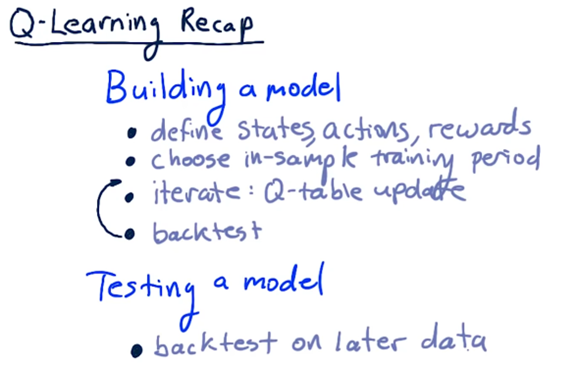
- Q-Learning Recap
What is Q
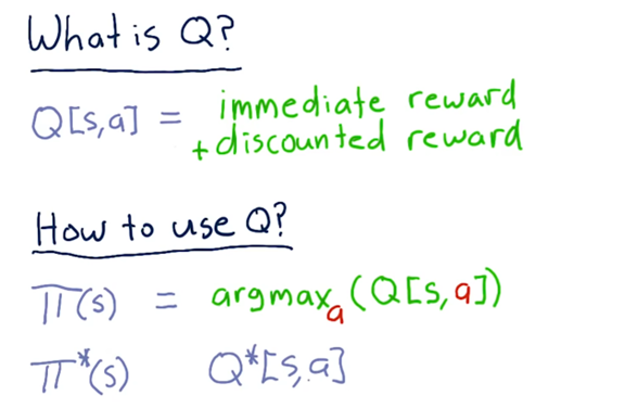
We know at a high level what Q-learning is, but what is Q? Q can either be written as a function,Q(s,a), or a table, Q[s,a]. In this class, we think of Q as a table. Regardless of the implementation, Q provides a measure of the value of taking an action, a, in a state, s.
The value that Q returns is actually the sum of two rewards: the immediate reward of taking a in s plus the discounted reward, the reward received for future actions. As a result, Q is not greedy; that is, it does not only consider the reward of acting now but also considers the value of actions down the road.
How to use Q
Remember that what we do in any particular state depends on the policy, π. Formally, π is a function that receives a state, s, as input and produces an action, a, as output.
We can leverage a Q-table to determine π. For a particular state, s, we can consult the Q-table and, across all possible actions, A, return the particular action, a, such that Q[s,a] is as large possible. Formally,
$$\pi(s)=argmax_a(Q[s,a]),a∈A$$
If we run Q-learning for long enough, we find that π(s) eventually converges to the optimal policy, which we denote as $π^{*}(s)$. Similarly, the optimal Q-table is $Q^{*}[s,a]$.
Learning Prodecure
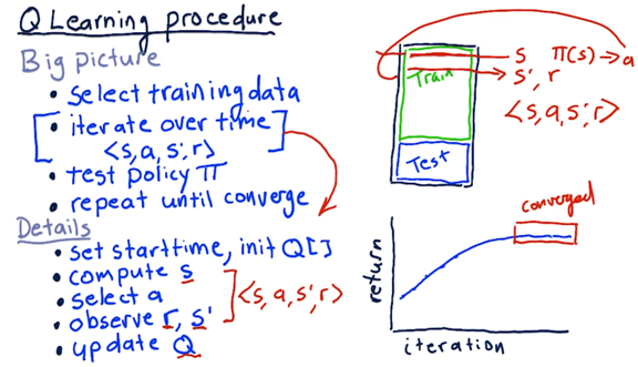
Recall how we partition our data for a machine learning problem: we need a larger training set and a somewhat smaller testing set. Since we are looking at stock features over time - our data set is a time series - we have to ensure that the dates in the training set precede those in the test set.
We then iterate through each time step in our training set. We evaluate a row of data to get our state, s. We then consult our policy, π, for that s to get an action, a. We execute that action and observe the resulting state, s′, and our reward, r.
For each training example, we produce an experience tuple, containing s, a, s′, and r. We use this tuple to update our Q-table, which effectively updates our policy.
Updating our Q-table requires us to have some semblance of a Q-table in place when we begin training. Usually, we initialize a Q-table with small random numbers, although various other initialization setups exist.
After we have finished iterating through our training data, we take the policy that we learned and apply it to the testing data. We mark down the performance and then repeat the entire process until the policy converges.
Update Rule
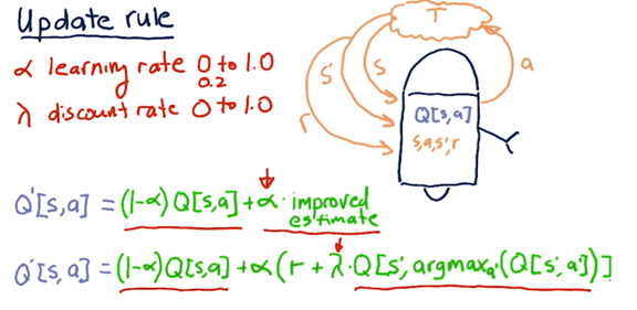
There are two components to the update rule. The first part concerns the current Q-value for the seen state and taken action:Q[s,a]. The second part concerns an improved estimate, E, of the Q-value. To combine the two, we introduce a new variable: α.
$$Q′[s,a]=(1-\alpha)*Q[s,a]+\alpha*E$$
We refer to α as the learning rate. It can take on any value between 0 and 1; typically, we use 0.2. Smaller values of α place more weight on the current Q-value, whereas larger values of α put more emphasis on E. We can think about this in another way: larger values of α make our robot learn more quickly than smaller values.
When we talk about the improved estimate, E, for the Q-value, we are talking about the sum of the current reward, r, and the future rewards, f. Remember that we have to discount future rewards, which we do with γ.
$$Q′[s,a]=(1-\alpha)*Q[s,a]+\alpha*(r+\gamma * f)$$
If we think about the future rewards, f, what we are looking for is the Q-value for the new state, s′. That is, the future reward for taking action a in state s is that action, a′, that maximizes the Q-value with regard to state s′.
$$Q′[s,a]=(1-\alpha)*Q[s,a]+\alpha*(r+\gamma * Q[s, argmax_{a′}(Q[s′,a′]))$$
Two Finner Points
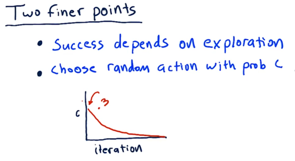
The success of Q-learning depends to a large extent on exploration. Exploration helps us learn about the possible states we can encounter as well as the potential actions we can take. We can use randomness to introduce exploration into our learning.
Instead of always selecting the action with the highest Q-value for a given state, we can, with some probability, decide to choose a random action. In this way, we can explore actions that our policy does not advise us to take to see if, potentially, they result in a higher reward.
A typical way to implement random exploration is to set the probability of choosing a random action to about 0.3 initially; then, over each iteration, we decay that probability steadily until we effectively don’t choose random actions at all.
The Trading Problem: Actions
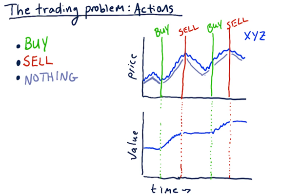
Now that we have a basic understanding of Q-learning, let’s see how we can turn the stock trading problem into a problem that Q-learning can solve. To do that, we need to define our actions, states, and rewards.
The model that we build is going to advise us to take one of three actions: buy, sell, or do nothing. Presumably, it is going to tell us to do nothing most of the time, with a few buys and sells scattered here and there.
The Trading Problem: Rewards Quiz
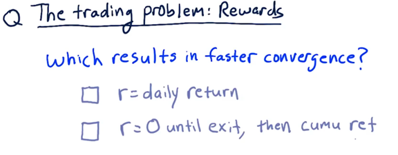
The rewards that our learner reaps should relate in some way to the returns of our strategy. There are at least two different ways that we can think about rewards.
On the one hand, we can think about the reward for a position as the daily return of a stock held in our portfolio. On the other hand, we can think about the reward for a position being zero until we exit the position, at which point the reward is the cumulative return of that position.
Which of these approaches results in a faster convergence to the optimal policy?
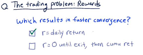
If we reward a little bit each day, the learner can learn much more quickly because it receives much more frequent rewards.
The Trading Problem: State Quiz
Consider the following factors and select which should be part of the state that we examine when selecting an appropriate action.
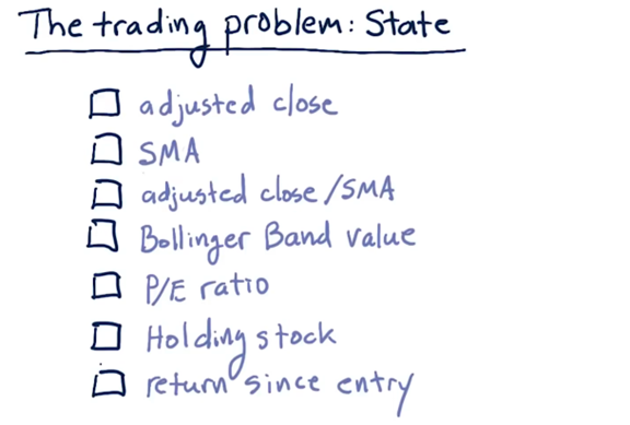
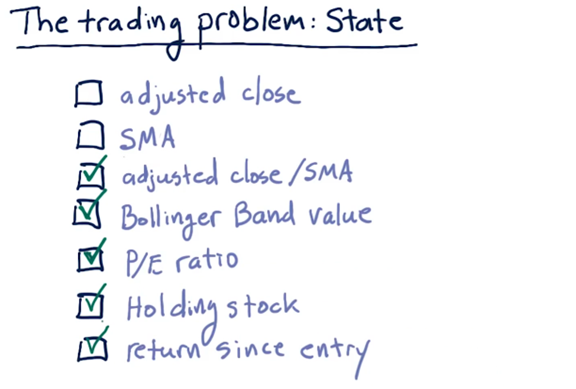
Neither adjusted close nor SMA alone are useful components of the state because they don’t particularly mean much as absolute values.
However, the ratio of adjusted close to SMA can be a valuable piece of state. For example, a positive ratio indicates that the close is larger than the SMA, which may be a sell signal. Additionally, other technical and fundamental indicators such as Bollinger Bands and P/E ratio can be essential parts of our state.
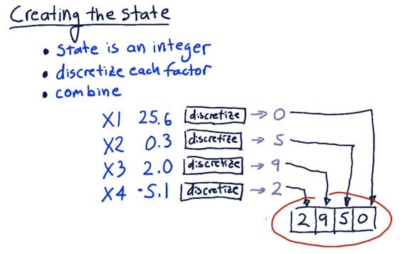
Creating the State
In Q-learning, we need to be able to represent our state as an integer; that way, we can use it to index into our Q-table, which is of finite dimension. Converting our state to an integer requires two steps.
First, we must discretize each factor, which essentially involves mapping a continuous value to an integer. Second, we must combine all of our discretized factors into a single integer that represents the overall state.
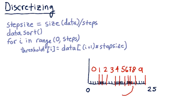
Discretizing
Discretization is a process by which we convert a real number into an integer across a limited scale. For example, for a particular factor, we might observe hundreds of different real values from 0 to 25. Discretization allows us to map those values onto a standardized scale of integers from, say, 0 to 9.
Let’s look at how we might discretize a set of data. The first thing we need to do is determine how many buckets we need. For example, if we want to map all values onto a number between 0 and 9, we need 10 buckets.
Next, we determine the size of our buckets, which is simply the total number of data elements divided by the number of buckets. For example, with 10 buckets and 100 data elements, our bucket size is 10.
Finally, we sort the data and determine the threshold for each bucket based on the step size. For example, with 10 buckets and 100 sorted data elements, our threshold for the discretized value, 1, is the tenth element, our threshold for the discretized value, 2, is the twentieth element, and so on.
A consequence of this approach is that when the data are sparse, the thresholds are set far apart. When the data is very dense, the thresholds end up being very close together.
Q-Learning Recap