- The RL Problem
- Mapping Trading to RL
- Markov Decision Problems
- Unknown Transitions and Rewards
- What to Optimize
- RL Summary
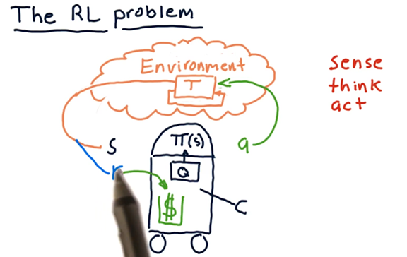
The RL Problem
To demonstrate one possible algorithm, let’s consider a robot interacting with the environment.
First, the robot observe the environment; more specifically, it reads in some representation of the environment. We call this representation the state, which we denote as S.
The robot has to process S to determine what action to take and does so by consulting a policy, which we denote as π. The robot considers S with regard to π and outputs an action a.
The action a changes the environment in some way, and we can use a transition function, denoted as T, to derive a new environment from the current environment and a particular action.
Naturally, the robot reads in the updated environment as a new S, against which it consults π to generate a new a. We refer to this circular process as the sense, think, act cycle.
To understand how the robot arrives at the policy π, we have to consider another component of this cycle: the reward, r. For any action that the robot takes, in any particular state, there is an associated reward.
As an example, if a navigation robot senses a cliff ahead and chooses to accelerate, the associated reward might be very negative. If, however, the robot chooses to turn around, the reward might be very positive.
In our case, we can imagine that our robot has a little wallet where it keeps its cash. The reward for a particular action might be how much cash that action adds to the wallet. The objective of this robot is to execute actions that maximize this reward.
Somewhere within the robot, there is an algorithm that synthesizes information about S, r, and a over time to generate π.
Trading as an RL Problem Quiz
We want to use reinforcement learning algorithms to trade; to do so, we have to translate the trading problem into a reinforcement learning problem.
Consider the following items. For each item, select whether the item corresponds to a component of the external state S, an action a we might take within the environment, or a reward r that we might use to inform our policy π.
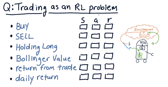
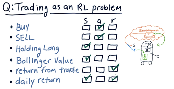
To be noticed here, daily return could be either a component of the state - a factor we consider before generating an action - but it could also be a reward.
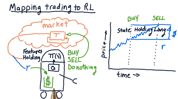
Mapping Trading to RL
Let’s think about how we can frame stock trading as an RL problem. In trading, our environment is the market. The state that we process considers, among other factors: market features, price information, and whether we are holding a particular stock. The actions we can execute within the environment are, generally, buy, sell, or do nothing.
In the context of buying a particular stock, we might process certain technical features - like Bollinger Bands - to determine what action to take. Suppose that we decide to buy a stock. Once we buy a stock, that holding becomes part of our state.
We have transitioned from a state of not holding to holding long through executing the buy action. We can transition from a state of holding long to not holding by executing the sell action.
Suppose the price increases, and we decide to execute a sell. The money that we made, or lost, is the reward that corresponds to the actions we took. We can use this reward and its relationship to the actions and the state to refine our policy, thus adjusting how we act in the environment.
Markov Decision Problems
A problem parameterized by set of states S, set of actions A, Transition function T, and reward funciton R is known as a Markov decision process.
The problem for a reinforcement learning algorithm is to find a policy π that maximizes reward over time. We refer to the theoretically optimal policy, which the learning algorithm may or may not find, as π∗.
Unknown Transitions and Rewards
Most of the time, we don’t know the transition function, T, or the reward function, R, a priori. As a result, the reinforcement learning agent has to interact with the world, observe what happens, and work with the experience it gains to build an effective policy.
Let’s say our agent observed state $s_1$, took action $a_1$, which resulted in state $s_1^{‘}$ and reward $r_1$. We refer to the object $(s_1, a_1, S_1^{‘}, r_1)$ as an experience tuple.
The agent iterates through this sense-think-act cycle over and over again, gathering experience tuples along the way. Once we have collected a significant number of these tuples, we can use two main types of approaches to find the appropriate policy,
π.
The first set of approaches is model-based reinforcement learning. In model-based reinforcement learning, we look at the experience tuples over time and build a model of T and R by examining the transitions statistically. For example, for each state, action pair $s_i, a_i$, we can look at the distributions of the observed next state and reward, $s_i^{‘}$ and $a_i^{‘}$, respectively. Once we have these models, we can use value iteration or policy iteration to find the policy.
The second set of approaches is model-free reinforcement learning. Model-free reinforcement learning methods derive a policy directly from the data. We are going to focus on Q-learning in this class, which is a specific type of model-free learning.
What to Optimize
We haven’t gone into much detail about what exactly we are trying to optimize; currently, we have a vague idea that we are trying to maximize the sum of our rewards. To make our discussion of optimization more concrete, consider our robot navigating the following maze.
Let’s say we wanted to optimize the sum of the robot’s rewards from now until infinity. We refer to this timeframe as an infinite horizon. In this case, we don’t particularly care if the robot exclusively grabs the 1 dolloar ad infinitum, or if it first grabs the 1 million dolloars before returning to the 1 dolloar. With regard to the reward, either strategy is sufficient since both result in an infinite reward.
More often than not, we have a finite horizon. We might, for example, want to optimize our reward over the next three moves. If we take three steps towards the 1 million reward, we are going to experience three penalties of -1, for a total penalty of -3. If we take three steps towards the 1 dolloar, however, we experience a reward of zero, a reward of 1 dolloar, and a reward of 0, for a total reward of 1 dolloar.
If we extend our horizon out to eight moves, we see that the optimal path changes. Instead of retrieving the 1 dolloar reward four times, we can incur seven penalties of -1 in exchange for the 1 million reward.
We can now articulate the expression that we want to maximize as shown in the figure.
The value of γ is greater than zero and less than or equal to one. The closer it is to one, the more we value rewards in the future (the less we discount them). The closer it is to zero, the less we value rewards in the future (the more we discount them).
Which Approach Gets $1M Quiz
Which of the following approaches leads our robot to a policy that causes it to reach the $1 million reward?
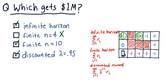
To be noticed here, in the discounted scenario, each reward in the future is successively devalued by 5%. Even so, the $1 million reward is so large that seeking this reward is still the optimal strategy.

